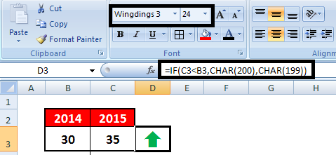
This tutorial explains how to create interactive up down arrows with excel.
Style 1 :
1. Enter CHAR(199) and change the font to "Wingdings 3", you will see Up arrow,
Style 1 :
| Image may be NSFW. Clik here to view.  |
| Interactive Up Down Arrow |
2. Enter CHAR(200) and change the font to "Wingdings 3", you will see Down arrow.
Next, apply conditional formatting
Click on "Next Rule" and select "Use a formula to determine which cells to format" and enter the following formula and click on "Format" and go to "Font" tab and select Red colorand then click on OK.
Style 2
1. Enter p and change the font to "Wingdings 3", you will see Up arrow,
Next, apply conditional formatting
Click on "Next Rule" and select "Use a formula to determine which cells to format" and enter the following formula and click on "Format" and go to "Font" tab and select Red colorand then click on OK.
=IF($D$3=CHAR(200),1,0)Create a new rule - Click on "Next Rule" and select "Use a formula to determine which cells to format" and enter the following formula and click on "Format" and go to "Font" tab and select Green color and then click on OK.
=IF($D$3=CHAR(199),1,0)
Style 2
| Image may be NSFW. Clik here to view.  |
| Style 2 : Up Down Arrow |
2. Enter q and change the font to "Wingdings 3", you will see Down arrow.
Next, apply conditional formatting
Click on "Next Rule" and select "Use a formula to determine which cells to format" and enter the following formula and click on "Format" and go to "Font" tab and select Red color and then click on OK.
Next, apply conditional formatting
Click on "Next Rule" and select "Use a formula to determine which cells to format" and enter the following formula and click on "Format" and go to "Font" tab and select Red color and then click on OK.
=IF($D$3="q",1,0)Create a new rule - Click on "Next Rule" and select "Use a formula to determine which cells to format" and enter the following formula and click on "Format" and go to "Font" tab and select Green color and then click on OK.
=IF($D$3="p",1,0)
