In this article, we will walk you through an application of topic modelling and sentiment analysis to solve a real world business problem. This approach has a onetime effort of building a robust taxonomy and allows it to be regularly updated as new topics emerge. This approach is widely used in topic mapping tools. Please note that this is not a replacement of the topic modelling methodologies such as Latent Dirichlet allocation (LDA) and it is beyond them.
Suppose you are head of the analytics team with a leading Hotel chain “Tourist Hotel”. Each day, you receive hundreds of reviews of your hotel on the company’s website and multiple other social media pages. The business has a challenge of scale in analysing such data and identify areas of improvements. You use a taxonomy based approach to identify topics and then use a built-in functionality of Python NLTK package to attribute sentiment to the comments. This will help you in identifying what the customers like or dislike about your hotel.
The customer review data consists of a serial number, an arbitrary identifier to identify each review uniquely and a text field that has the customer review.
Steps to topic mapping and sentiment analysis
1. Identify Topics and Sub Topics
2. Build Taxonomy
3. Map customer reviews to topics
4. Map customer reviews to sentiment
Step 1 : Identifying Topics
II. Build Keywords
The taxonomy is built in a CSV file format. There are 3 levels of key words for each sub topic namely, Primary key words, Additional key words and Exclude key words. The keywords for the topics need to be manually identified and added to the taxonomy file. The TfIDf, Bigram frequencies and LDA methodologies can help you in identifying the right set of keywords. Although there is no one best way for building key words, below is a suggested approach.
i. Primary key words are the key words that are mostly specific to the topic. These key words need to be mutually exclusive across different topics as far as possible.
ii. Additional key words are specific to the sub topic. These key words need not be mutually exclusive between the topics but it is advised to maintain exclusivity between sub topics under the same sub topic. To explain further, let us say, there is a sub topic “Price” under the topics “Room” as well as “Food”, then the additional key words will have an overlap. This will not create any issue as the primary key words are mutually exclusive.
iii. Exclude key words are key words that are used relatively less than the other two types. If there are two sub topics that have some overlap of additional words OR for example, if the sub topic “booking” is incorrectly mapping comments regarding taxi bookings as room booking, such key words could be used in exclude words to solve the problem.
Benefits of using taxonomic approach
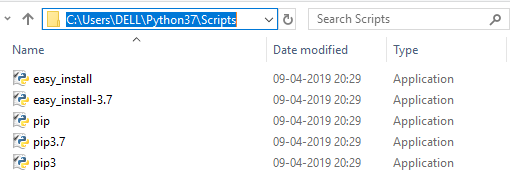
Below is the python code that helps in mapping reviews to categories. Firstly, import all the libraries needed for this task. Install these libraries if needed.
Download Datafiles
Customer Review
Taxonomy
Import reviews data
Build functions for handling the various repetitive tasks during the mapping exercise. This function identifies taxonomy words ending with (*) and treats it as a wild character. This takes the Keywords as input and uses regular expression to identify all the other keyword matches as output.
Function to remove just the quotes(""). This is different from the above as this only handles double quotes. Recall that we wrap phrases or key words with special characters in double quotes.
Split each document by sentences and append one below the other for sentence level topic mapping.
Step 4: Map customer reviews to sentiment
Output the sentiment mapped data
Polarity Scoring Explained:
NLTK offers Valence Aware Dictionary for sEntiment Reasoning(VADER) model that helps in identifying both the direction (polarity) as well as the magnitude(intensity) of the text. Below is the high-level explanation of the methodology.
VADER is a combination of lexical features and rules to identify sentiment and intensity. Hence, this does not need any training data. To explain further, if we take an example of the sentence “the food is good”, it is easy to identify that it is positive in sentiment. VADER goes a step ahead and identifies intensity based on rule based approach such as punctuation, capitalised words and degree modifications.
The polarity scores for the different variations of similar sentences is as follows:
Although VADER works well on multiple domains, there are could be some domains where it is preferred to build one’s own sentiment training models. Below are the two examples of such use cases.
 |
| Text Mining Case Study using Python |
Case Study : Topic Modeling and Sentiment Analysis
Data Structure
The customer review data consists of a serial number, an arbitrary identifier to identify each review uniquely and a text field that has the customer review.
 |
| Example : Sentiment Analysis |
Steps to topic mapping and sentiment analysis
1. Identify Topics and Sub Topics
2. Build Taxonomy
3. Map customer reviews to topics
4. Map customer reviews to sentiment
Step 1 : Identifying Topics
The first step is to identify the different topics in the reviews. You can use simple approaches such as Term Frequency and Inverse Document Frequency or more popular methodologies such as LDA to identify the topics in the reviews. In addition, it is a good practice to consult a subject matter expert in that domain to identify the common topics. For example, the topics in the “Tourist Hotel” example could be “Room booking”, “Room Price”, “Room Cleanliness”, “Staff Courtesy”, “Staff Availability ”etc.
Step 2 : Build Taxonomy
I. Build Topic Hierarchy
I. Build Topic Hierarchy
Based on the topics from Step 1, Build a Taxonomy. A Taxonomy can be considered as a network of topics, sub topics and key words.
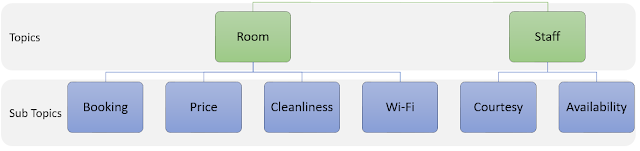 |
| Topic Hierarchy |
The taxonomy is built in a CSV file format. There are 3 levels of key words for each sub topic namely, Primary key words, Additional key words and Exclude key words. The keywords for the topics need to be manually identified and added to the taxonomy file. The TfIDf, Bigram frequencies and LDA methodologies can help you in identifying the right set of keywords. Although there is no one best way for building key words, below is a suggested approach.
i. Primary key words are the key words that are mostly specific to the topic. These key words need to be mutually exclusive across different topics as far as possible.
ii. Additional key words are specific to the sub topic. These key words need not be mutually exclusive between the topics but it is advised to maintain exclusivity between sub topics under the same sub topic. To explain further, let us say, there is a sub topic “Price” under the topics “Room” as well as “Food”, then the additional key words will have an overlap. This will not create any issue as the primary key words are mutually exclusive.
iii. Exclude key words are key words that are used relatively less than the other two types. If there are two sub topics that have some overlap of additional words OR for example, if the sub topic “booking” is incorrectly mapping comments regarding taxi bookings as room booking, such key words could be used in exclude words to solve the problem.
Snapshot of sample taxonomy:

Note: while building the key word list, you can put an “*” at the end as it helps as wild character. For example, all the different inflections of “clean” such as “cleaned”, “cleanly”, “cleanliness” can be handled by one keyword “clean*”. If you need to add a phrase or any keyword with a special character in it, you can wrap it in quotes. For example, “online booking”, Wi-Fi” etc need to be in double quotes.
Benefits of using taxonomic approach
Topic modelling approaches identify topics based on the keywords that are present in the content. For novel keywords that are similar to the topics but may come up in the future are not identified. There could be use cases where businesses want to track certain topics that may not always be identified as topics by the topic modelling approaches.
Step 3 : Map customer reviews to topic
Each customer comment is mapped to one or more sub topics. Some of the comments may not be mapped to any comment. Such instances need to be manually inspected to check if we missed any topics in the taxonomy so that it can be updated. Generally, about 90% of the comments have at least one topic. The rest of the comments could be vague. For example: “it was good experience” does not tell us anything specific and it is fine to leave it unmapped.
Each customer comment is mapped to one or more sub topics. Some of the comments may not be mapped to any comment. Such instances need to be manually inspected to check if we missed any topics in the taxonomy so that it can be updated. Generally, about 90% of the comments have at least one topic. The rest of the comments could be vague. For example: “it was good experience” does not tell us anything specific and it is fine to leave it unmapped.
Snapshot of how the topics are mapped:
 |
| Topic Mapping |
Below is the python code that helps in mapping reviews to categories. Firstly, import all the libraries needed for this task. Install these libraries if needed.
import pandas as pd
import numpy as np
import re
import string
import nltk
from nltk.tokenize import word_tokenize
from nltk.sentiment.vader import SentimentIntensityAnalyzer
Download Datafiles
Customer Review
Taxonomy
Import reviews data
df = pd.read_csv("D:/customer_reviews.csv");
Import taxonomy
df_tx = pd.read_csv("D:/ taxonomy.csv");
Build functions for handling the various repetitive tasks during the mapping exercise. This function identifies taxonomy words ending with (*) and treats it as a wild character. This takes the Keywords as input and uses regular expression to identify all the other keyword matches as output.
def asterix_handler(asterixw, lookupw):This function removes all punctuations. This is helpful in terms of data cleaning. You can edit the list of punctuations for your own custom punctuation removal at the place highlighted in amber.
mtch = "F"
for word in asterixw:
for lword in lookupw:
if(word[-1:]=="*"):
if(bool(re.search("^"+ word[:-1],lword))==True):
mtch = "T"
break
return(mtch)
def remov_punct(withpunct):
punctuations = '''!()-[]{};:'"\,<>./?@#$%^&*_~'''
without_punct = ""
char = 'nan'
for char in withpunct:
if char not in punctuations:
without_punct = without_punct + char
return(without_punct)
Function to remove just the quotes(""). This is different from the above as this only handles double quotes. Recall that we wrap phrases or key words with special characters in double quotes.
def remov_quote(withquote):
quote = '"'
without_quote = ""
char = 'nan'
for char in withquote:
if char not in quote:
without_quote = without_quote + char
return(without_quote)
Split each document by sentences and append one below the other for sentence level topic mapping.
sentence_data = pd.DataFrame(columns=['slno','text'])Drop empty text rows if any and export data
for d in range(len(df)):
doc = (df.iloc[d,1].split('.'))
for s in ((doc)):
temp = {'slno': [df['slno'][d]], 'text': [s]}
sentence_data= pd.concat([sentence_data,pd.DataFrame(temp)])
temp = ""
sentence_data['text'].replace('',np.nan,inplace=True);
sentence_data.dropna(subset=['text'], inplace=True);

data = sentence_data
cat2list = list(set(df_tx['Subtopic']))
#data = pd.concat([data,pd.DataFrame(columns = list(cat2list))])
data['Category'] = 0
mapped_data = pd.DataFrame(columns = ['slno','text','Category']);
temp=pd.DataFrame()
for k in range(len(data)):
    comment = remov_punct(data.iloc[k,1])
data_words = [str(x.strip()).lower() for x in str(comment).split()]
data_words = filter(None, data_words)
    output = []

    for l in range(len(df_tx)):
key_flag = False
and_flag = False
not_flag = False
        if (str(df_tx['PrimaryKeywords'][l])!='nan'):
kw_clean = (remov_quote(df_tx['PrimaryKeywords'][l]))
        if (str(df_tx['AdditionalKeywords'][l])!='nan'):
aw_clean = (remov_quote(df_tx['AdditionalKeywords'][l]))
        else:
aw_clean = df_tx['AdditionalKeywords'][l]
        if (str(df_tx['ExcludeKeywords'][l])!='nan'):
nw_clean = remov_quote(df_tx['ExcludeKeywords'][l])
        else:
nw_clean = df_tx['ExcludeKeywords'][l]
Key_words = 'nan'
and_words = 'nan'
        and_words2 = 'nan'
not_words = 'nan'
        not_words2 = 'nan'

        if(str(kw_clean)!='nan'):
key_words = [str(x.strip()).lower() for x in kw_clean.split(',')]
            key_words2 = set(w.lower() for w in key_words)

        if(str(aw_clean)!='nan'):
and_words = [str(x.strip()).lower() for x in aw_clean.split(',')]
            and_words2 = set(w.lower() for w in and_words)

        if(str(nw_clean)!= 'nan'):
not_words = [str(x.strip()).lower() for x in nw_clean.split(',')]
            not_words2 = set(w.lower() for w in not_words)

        if(str(kw_clean) == 'nan'):
key_flag = False
        else:
            if set(data_words) & key_words2:
key_flag = True
            else:
if(asterix_handler(key_words2, data_words)=='T'):
key_flag = True

        if(str(aw_clean)=='nan'):
and_flag = True
        else:
            if set(data_words) & and_words2:
and_flag = True
            else:
                if(asterix_handler(and_words2,data_words)=='T'):
and_flag = True
        if(str(nw_clean) == 'nan'):
not_flag = False
        else:
            if set(data_words) & not_words2:
not_flag = True
            else:
if(asterix_handler(not_words2, data_words)=='T'):
not_flag = True
if(key_flag == True and and_flag == True and not_flag == False):
output.append(str(df_tx['Subtopic'][l]))
            temp = {'slno': [data.iloc[k,0]], 'text': [data.iloc[k,1]], 'Category': [df_tx['Subtopic'][l]]}
mapped_data = pd.concat([mapped_data,pd.DataFrame(temp)])
    #data['Category'][k] = ','.join(output)

#output mapped data
mapped_data.to_csv("D:/ mapped_data.csv",index = False)
Step 4: Map customer reviews to sentiment
#read category mapped data for sentiment mapping#Build a function to leverage the built-in NLTK functionality of identifying sentiment. The output 1 means positive, 0 means neutral and -1 means negative. You can choose your own set of thresholds for positive, neutral and negative sentiment.
catdata = pd.read_csv("D:/mapped_data.csv")
def findpolar(test_data):
sia = SentimentIntensityAnalyzer()
    polarity = sia.polarity_scores(test_data)["compound"];
if(polarity >= 0.1):
foundpolar = 1
if(polarity <= -0.1):
foundpolar = -1
    if(polarity>= -0.1 and polarity<= 0.1):
foundpolar = 0
    return(foundpolar)
Output the sentiment mapped data
catdata.to_csv("D:/sentiment_mapped_data.csv",index = False)
 |
| Output : Sentiment Analysis |
Additional Reading
Polarity Scoring Explained:
NLTK offers Valence Aware Dictionary for sEntiment Reasoning(VADER) model that helps in identifying both the direction (polarity) as well as the magnitude(intensity) of the text. Below is the high-level explanation of the methodology.
VADER is a combination of lexical features and rules to identify sentiment and intensity. Hence, this does not need any training data. To explain further, if we take an example of the sentence “the food is good”, it is easy to identify that it is positive in sentiment. VADER goes a step ahead and identifies intensity based on rule based approach such as punctuation, capitalised words and degree modifications.
The polarity scores for the different variations of similar sentences is as follows:
 |
| Polarity Score |
Use cases where training sentiment models is suggested over Sentiment Intensity Analyzer:
Although VADER works well on multiple domains, there are could be some domains where it is preferred to build one’s own sentiment training models. Below are the two examples of such use cases.
- Customer reviews on alcoholic beverages: It is common to observe people using otherwise negative sentiment words to describe positive experience. For example, the sentence “this sh*t is fu**ing good” means that this drink is good but VADER approach gives it a “-10” suggesting negative sentiment
- Patient reviews regarding hospital treatment Patient’s description of their problem is a neutral sentiment but VADER approach considers it as negative sentiment. For example, the sentence “I had an unbearable back pain and your medication cured me in no time” is given “-0.67” suggesting negative sentiment.