Quantcast
Channel: ListenData
Viewing all 425 articles
Browse latest View live

Two Sample Ttest with R

$
0
0
In this tutorial, we will cover how to run two sample t-test with R.

Two Sample Ttest with R
Introduction : Significance Testing
You have a sample data and you are asked to assess the credibility of a statement about population. Statistical significance evaluates the likelihood that an observed difference is due to chance.

It deals with the following questions :
If we selected many samples from the same population, would we still find the same relationship between these two variables in every sample? Or is our finding due only to random chance?
Independent Two Sample T-Test

The independent t test evaluates whether the means for two independent groups are significantly different from each other. It is used for just 2 groups of samples. If you have more than 2 groups of samples, you should use ANOVA. For example, if we compare mean salary of male and female employees and check whether there is a statistical significant difference between the mean salary between them.

Assumptions of Independent Sample T-Test
  1. Each score is sampled independently and randomly. 
  2. The scores are normally distributed within each of the two groups.
  3. The variance in each of the groups is equal.

Mathematical Formula

Two Sample t-test Formula

x1-bar and x2-bar are sample means and sample sizes : n1 and n2. Unknown population means- mu1-bar and mu2-bar. s1 and s2 are sample standard deviations.

Dependent (or Paired) Two Sample T-Test
The paired t test compares the means of two groups that are correlated. In other words, it evaluates whether the means for two paired groups are significantly different from each other.  This paired t-test is used in ‘before-after’ studies, or 'case-control' studies.  Example, if we give training to students about R-Programming language and we want to see whether or not the training had any impact on the students' score on R-programming test, we could use the paired sample test.

Assumptions of Paired T-Test
  1. Only the paired groups can be used to perform the paired test.
    1. Each score is sampled independently and randomly. 
    2. The scores are normally distributed within each of the two groups.
    3. The variance in each of the groups is equal.

    Type I and II Errors

    Hypothesis Testing : Type I and II Errors

    Case Study [Independent Sample T-Test]

    Of year 2009 Psychology major students, each student in a random sample of 200 students was asked how many statistics classes they were enrolled in.

    Of year 2015 Psychology major students, each student in a random sample of 200 students was asked how many statistics classes they were enrolled in.

    We wanted to see whether the mean number of enrollment in statistics classes has changed over the past 6 years.

    Solution : Independent T-Test
    Since students from batch of 2009 and 2015 are not same, we should use Independent T-test rather than Paired T-test.

    Null Hypothesis

    It is a statement that you want to test. It usually states that there is no relationship between the two variables.

    In this case, the null hypothesis states that there is no difference between the mean number of enrollment in statistics classes in 2009 and 2015 batch.

    Alternate Hypothesis

    It is contrary to the null hypothesis. It usually states that there is a relationship between the two variables.

    In this case, the alternate hypothesis states that there is a difference between the mean number of enrollment in statistics classes in 2009 and 2015 batch.


    Create Sample Data in R


    1. Define Sample I

    batch2009 <- c(rep(1,14), rep(2,48), rep(3,60), rep(4,38), rep(5,26), rep(6,14))
    table(batch2009)

    2. Define Sample II
    batch2015 <- c(rep(1,20), rep(2,32), rep(3,60), rep(4,40), rep(5,26), rep(6,22))
    table(batch2015)

    Visualize Groups
    Sample I Data
    Sample II Data


    R Code : Two Sample Ttest
    t.test(batch2009, batch2015, var.equal=FALSE)
    When the var.equal argument is set to FALSE in the above syntax, it runs Welch's two sample t-test.
    Welch Two Sample T-test
    Since p-value is greater than 0.05, it means we fail to reject the null hypothesis. It implies there is no significant difference between the mean number of enrollment in statistics class in batch 2009 and batch 2015.

    Should i check Assumption : Equality Of Variance?

    Most of the stats textbooks recommends we should first test the assumption that variances are equal with Levene’s test. However, most of the whitepapers proves that in simulation of several studies, levene’s test fails to reject the null-hypothesis that variances are equal even when variances are unequal. Hence, we should always use Welch's two sample t-test.
    Welch's t-test performs better than Student's t-test whenever sample sizes and variances are unequal between groups, and gives the same result when sample sizes and variances are equal.
    In case you are interested to run Levene Test for Equality of Variance, check the following program :
    temp = rbind(data.frame(x=batch2009, group=1), data.frame(x=batch2015, group=2))
    temp$group = as.factor(temp$group)
    library(car)
    leveneTest(temp$x, group = temp$group, center = mean)
    In this example, the significance (p value) of Levene's test is 0.2003. Since this value is greater than 5% level of significance (0.05), we fail to reject the null hypothesis that the variability of the two groups is equal, implying that the variances are unequal.

    Run T-test of Equal Variance :
    t.test(batch2009, batch2015, var.equal=TRUE)
    It returns the same result as shown above in the Welch's Sample T-test result.

    How to calculate t-test and p-value manually
    xhat1 <- mean(batch2009)
    xhat2 <- mean(batch2015)
    s1 <- sd(batch2009)
    s2 <- sd(batch2015)
    n1 <- length(batch2009)
    n2 <- length(batch2015)
    diff_in_means <- xhat1 - xhat2
    SE_diff_mean <- sqrt(s1^2/n1+s2^2/n2)
    t_stat <- diff_in_means/SE_diff_mean
    t_stat
    pvalue = 2* pt(t_stat, df=n1+n2-2)
    pvalue

    Complete Guide to PROC UNIVARIATE

    $
    0
    0
    This tutorial explains how to explore data with PROC UNIVARIATE. It is one of the most powerful SAS procedure for running descriptive statistics as well as checking important assumptions of various statistical techniques such as normality, detecting outliers. Despite various powerful features supported by PROC UNIVARIATE, its popularity is low as compared to PROC MEANS. Most of the SAS Analysts are comfortable running PROC MEANS to run summary statistics such as count, mean, median, missing values etc, In reality, PROC UNIVARIATE surpass PROC MEANS in terms of options supported in the procedure. See the main difference between the two procedures.

    PROC UNIVARIATE vs. PROC MEANS

    1. PROC MEANS can calculate various percentile points such as 1st, 5th, 10th, 25th, 50th, 75th, 90th, 95th, 99th percentiles but it cannot calculate custom percentiles such as 20th, 80th, 97.5th, 99.5th percentiles. Whereas, PROC UNIVARIATE can run custom percentiles.

    2. PROC UNIVARIATE can calculate extreme observations - the five lowest and five highest values. Whereas, PROC MEANS can only calculate MAX value.

    3. PROC UNIVARIATE supports normality tests to check normal distribution. Whereas, PROC MEANS does not support normality tests.

    4. PROC UNIVARIATE generates multiple plots such as histogram, box-plot, steam leaf diagrams whereas PROC MEANS does not support graphics.


    Basic PROC UNIVARIATE Code

    In the example below. we would use sashelp.shoes dataset. SALES is the numeric (or measured) variable.
    proc univariate data = sashelp.shoes;
    var sales;
    run;
    Default Output of PROC UNIVARIATE

    1. Moments : Count, Mean, Standard Deviation, SUM etc

    2. Basic Statistics : Mean, Median, Mode etc

    Default Output : PART I

    3. Tests for Location : one-sample t-test, Signed Rank test.

    4. Percentiles (Quantiles)

    5. Extreme Observations - first smallest and largest values against their row position.
    Default Output : Part II

    Example 1 : Analysis of Sales by Region

    Suppose you are asked to calculate basic statistics of sales by region. In this case, region is a grouping (or categorical) variable. The CLASS statement is used to define categorical variable.
    proc univariate data = sashelp.shoes;
    var sales;
    class region;
    run;
    See the output shown below -
    PROC UNIVARIATE Class Statement
     The similar output was generated for other regions - Asia, Canada, Eastern Europe, Middle East etc.

    2. Generating only Percentiles in Output

    Suppose you want only percentiles to be appeared in output window. By default, PROC UNIVARIATE creates five output tables : Moments, BasicMeasures, TestsForLocation, Quantiles, and ExtremeObs. The ODS SELECT can be used to select only one of the table. The Quantiles is the standard table name of PROC UNIVARIATE for percentiles which we want. ODS stands for Output Delivery System.
    ods select Quantiles;
    proc univariate data = sashelp.shoes;
    var sales;
    class region;
    run;
    How to know the table names generated by SAS procedure

    The ODS TRACE ON produces name and label of tables that SAS Procedures generates in the log window.
    ods trace on;
    proc univariate data = sashelp.shoes;
    var sales;
    run;
    ods trace off;
    How to write Percentile Information in SAS Dataset

    The ODS OUTPUT statement is used to write output in results window to a SAS dataset. In the code below, temp would be the name of the dataset in which all the percentile information exists.
    ods output Quantiles = temp;
    proc univariate data = sashelp.shoes;
    var sales;
    class region;
    run;
    ods output close;

    3. Calculating Extreme Values

    Like we generated percentiles in the previous example, we can generate extreme values with extremeobs option. The ODS OUTPUT tells SAS to write the extreme values information to a dataset named outlier. The "extremeobs"is the standard table name of PROC UNIVARIATE for extreme values. 
    ods output extremeobs = outlier;
    proc univariate data = sashelp.shoes;
    var sales;
    class region;
    run;
    ods output close;
    4. Checking Normality

    Most of the statistical techniques assumes data should be normally distributed. It is important to check this assumption before running a model.

    There are multiple ways to check Normality :
    1. Plot Histogram and see the distribution
    2. Calculate Skewness
    3. Normality Tests

    I. Plot Histogram

    Histogram shows visually whether data is normally distributed.
    proc univariate data=sashelp.shoes NOPRINT;
    var sales;
    HISTOGRAM / NORMAL (COLOR=RED);
    run;
    It also helps to check whether there is an outlier or not.

    II. Skewness

    Skewness is a measure of the degree of asymmetry of a distribution. If skewness is close to 0, it means data is normal.

    Skewness
    A positive skewed data means that there are a few extreme large values which turns its mean to skew positively. It is also called right skewed.
    Positive Skewness : If skewness > 0, data is positively skewed. Another way to see positive skewness : Mean is greater than median and median is greater than mode.
    A negative skewed data means that there are a few extreme small values which turns its mean to skew negatively. It is also called left skewed.
    Negative Skewness : If skewness < 0, data is negatively skewed. Another way to see negative skewness : Mean is less than median and median is less  than mode.
    Rule :
    1. If skewness < −1 or > +1, the distribution is highly skewed.
    2. If skewness is between −1 and −0.5 or between 0.5 and +1, the distribution is moderately skewed.
    3. If skewness > −0.5 and  <  0.5, the distribution is approximately symmetric or normal.
    ods select Moments;
    proc univariate data = sashelp.shoes;
    var sales;
    run;
    Skewness and Normality
    Since Skewness is greater than 1, it means data is highly skewed and non-normal.


    III. Normality Tests

    The NORMAL keyword tells SAS to generate normality tests.
    ods select TestsforNormality;
    proc univariate data = sashelp.shoes normal;
    var sales;
    run;
    Tests for Normality

    The two main tests for normality are as follows :

    1. Shapiro Wilk Test [Sample Size <= 2000]
    It states that the null hypothesis - distribution is normal.
    In the example above, p value is less that 0.05 so we reject the null hypothesis. It implies distribution is not normal. If p-value > 0.05, it implies distribution is normal.
    This test performs well in small sample size up to 2000.

    2. Kolmogorov-Smirnov Test [Sample Size > 2000]

    In this test, the null hypothesis states the data is normally distributed.
    If p-value > 0.05, data is normal. In the example above, p-value is less than 0.05, it means data is not normal.
    This test can handle larger sample size greater than 2000.

    5. Calculate Custom Percentiles

    With PCTLPTS= option, we can calculate custom percentiles. Suppose you need to generate 10, 20, 30, 40, 50, 60, 70, 80, 90, 100 percentiles.
    proc univariate data = sashelp.shoes noprint;
    var sales;
    output out = temp
    pctlpts = 10 to 100 by 10 pctlpre = p_;
    run;
    The OUTPUT OUT= statement is used to tell SAS to save the percentile information in TEMP dataset. The PCTLPRE= is used to add prefix in the variable names for the variable that contains the PCTLPTS= percentile.

    Suppose you want to calculate 97.5 and 99.5 percentiles.
    proc univariate data = sashelp.shoes noprint;
    var sales;
    output out = temp
    pctlpts = 97.5,99.5 pctlpre = p_;
    run; 

    6.  Calculate Winsorized and Trimmed Means

    The Winsorized and Trimmed Means are insensitive to Outliers. They should be reported rather than mean when the data is highly skewed.

    Trimmed Mean : Removing extreme values and then calculate mean after filtering out the extreme values. 10% Trimmed Mean means calculating 10th and 90th percentile values and removing values above these percentile values.

    Winsorized Mean : Capping extreme values and then calculate mean after capping extreme values at kth percentile level. It is same as trimmed mean except removing the extreme values, we are capping at kth percentile level.

    Winsorized Mean

    In the example below, we are calculating 20% Winsorized Mean.
    ods select winsorizedmeans;
    ods output winsorizedmeans=means;
    proc univariate winsorized = 0.2 data=sashelp.shoes;
    var sales;
    run;
    Winsorized Means
    Percent Winsorized in Tail : 20% of values winsorized from each tail (upper and lower side)
    Number Winsorized in Tail : 79 values winsorized from each tail


    Trimmed Mean

    In the example below, we are calculating 20% trimmed Mean.
    ods select trimmedmeans;
    ods output trimmedmeans=means;
    proc univariate trimmed = 0.2 data=sashelp.shoes;
    var sales;
    run;

    7. Calculate Sample T-test

    It tests the null hypothesis that mean of the variable is equal to 0. The alternative hypothesis is that mean is not equal to 0. When you run PROC UNIVARIATE, it defaults generates sample t-test in 'Tests for Location' section of output.
    ods select TestsForLocation;
    proc univariate data=sashelp.shoes;
    var sales;
    run;

    Since p-value is less than 0.05. we reject the null hypothesis. It concludes the mean value of the variable is significantly different from zero.

    Ttest with PROC Univariate

    8. Generate Plots

    PROC UNIVARIATE generates the following plots :
    1. Histogram
    2. Box Plot
    3. Normal Probability Plot

      The PLOT keyword is used to generate plots.
      proc univariate data=sashelp.shoes PLOT;
      var sales;
      run;

      4 ways to calculate LAG and LEAD in SAS

      $
      0
      0
      This tutorial demonstrates multiple ways to calculate lag and lead in SAS. In time series data, it is generally required to calculate lag and lead of one or more measured variables. Time series or longitudinal data are considered one of the most challenging data manipulation tasks. This tutorial covers various data manipulation tricks to make it easy.

      What is Lag ?
      Looking back some number of periods or rows.
      Lag of first order - Looking back 1 observation (last value). It is denoted by lag1_value in the image shown below.
      Lag of second order - Looking back 2 observations. It is denoted by lag2_value in the image shown below.
      Calculate Lag in SAS

      Create a Sample Data

      The program below creates a sample data for demonstration.
      data example;
      input id value;
      cards;
      1 25
      1 30
      1 35
      1 40
      2 25
      2 30
      2 37
      ;
      run;
       LAG Function

      In SAS, the LAG function is used to compare the current value to its predecessors. If you want to calculate lag of second order, use LAG2 function. Similarly, you can use LAG3 function for measuring lag of third order.
      data temp;
      set example;
      lag1_value = lag(value);
      lag2_value = lag2(value);
      run;

      Calculating LAG by ID Variable

      Suppose you are asked to calculate LAG of first order by a grouping variable. In this case, there is no SAS function directly available to accomplish this task. We need to apply some tricks to make it happen.

      Method I : LAG and FIRST.

      The program below uses BY statement and FIRST. to measure lag of first order by ID. First, we are calculating lag and then make the value missing against the first record in a group i.e. ID.
      data temp;
      set example;
      by id;
      lag_value = lag(value);
      if first.id then lag_value = .;
      run;
      Lag by Group

      Method 2 : POINT=, NOBS and _N_

      The POINT= Option is used to point to a specified row number. The _N_ system variable is used to generate a serial number which are used as an index. The NOBS option is used to calculate the number of rows in a variable.
      data example;
      set example;
      lagid = lag(id);
      run;

      data lags;
       if _n_ <= k then do;
       set example point = _n_;
       if lagid = id then do;
       N = _N_ - 1;
       set example point = N;
       lag_value = value;
       end;
       end;
       else lag_value = .;
       set example nobs = k;
       by id;
       drop lagid;
       run;

      Method 3 : PROC SQL and FIRST.

      In the program below, we are first creating a sequence of values and later we are joining two tables taking primary key as current value from the first table with predecessor value from the second table.
      data example;
      set example;
      by id;
      if first.id then N = 1;
      else N + 1;
      run;
      proc sql;
      select a.* , b.value as lag_value
      from example a left join example b
      on a.id = b.id and a.N = b.N + 1;
      quit;

      Method 4 : PROC EXPAND

      PROC EXPAND is one of the most useful procedure of SAS ETS. It has multiple functions such as creating lag, lead and moving average variables by group(s), aggregation of previous k rows etc.
      proc expand data= example out= t2;
      convert value = lag_value /transformout = (lag 1);
      by id;
      run;
      It requires license of SAS ETS package.

      What is Lead?
      Looking ahead some number of rows or periods.
      Lead Value of First Order - Looking ahead one observation of  a variable (next row).
      Lead Value of Second Order - Looking ahead two observations of  a variable (next to next row).

      Lead Value

      Calculating Lead in SAS

      In SAS, there is no direct function for calculating LEAD. I feel the same there should be a SAS function for it :-) It can be calculated with the following logic :

      Create a sequence of numbers and then sort the sequence by descending order. Then we calculate lag of the variable for which we need to calculate lead. At last, we sort the data by sequence ID.

      data temp;
      set example;
      x + 1;
      run;

      proc sort data = temp;
      by descending x;
      run;

      data temp2;
      set temp;
      lead_value = lag(value);
      run;

      proc sort data = temp2;
      by x;
      run;


      Method 2 : POINT=, _N_ and NOBS

      The NOBS option counts the number of rows in a variable. The _N_+ 1 creates a sequence of numbers start from 2 to (number of records + 1). The POINT= points to a row when the sequence of numbers are less than or equal to number of rows.
      data temp;
      _N_+1;
      if _N_ <= k then do;
      set example point=_N_;
      lead_value = value;
      end;
      else lead_value = .;
      set example nobs=k;
      proc print noobs;
      run;
      Calculating Lead by ID Variable

      Method I : FIRST. and PROC SORT

      In this case, we are applying the same trick that we have used above to calculate lead. The only difference is we need to incorporate grouping variable to calculate lead by a grouping variable (ID).
      data temp;
      set example;
      by id;
      if first.id then x =1;
      else x + 1;
      run;

      proc sort data = temp;
      by id descending x;
      run;

      data temp2;
      set temp;
      by id descending x;
      l = lag(x);
      lead_val = lag(value);
      if first.id then do;
      l = .;
      lead_val = .;
      end;
      run;

      proc sort data = temp2;
      by id x;
      run;
      Lead Variables

      Method II : FIRST. and PROC SQL

      In the program below, we are performing self joins on next value with the current value.
      data example;
      set example;
      by id;
      if first.id then N = 1;
      else N + 1;
      run;

      proc sql;
      select a.* , b.value as lag_value
      from example a left join example b
      on a.id = b.id and a.N + 1 = b.N;
      quit;

      Method III : POINT= and NOBS

      In the program below, we have used the same POINT= and NOBS trick that we have used in the above article.
      data example;
       set example;
       lagid = lag(id);
      run;  
      data leads;
       _n_ + 1;
       if _n_ <= n then do;
       set example point=_n_;
       if lagid = id then do;
       y = value;
       end;
       end;
       else y = .;
       set example nobs = n;
       by id;
       drop lagid;
       proc print noobs;
       run;

      Method IV : PROC EXPAND

      PROC EXPAND can be used to calculate leads by a grouping variable. It can also calculate moving averages.
      proc expand data= example out= t2;
      convert value = lead_value /transformout = (lead 1);
      by id;
      run;
      The above method works only if you have a license of SAS ETS package.

      dplyr Tutorial

      $
      0
      0
      It's a complete tutorial on data analysis or manipulation with R. This tutorial covers one of the most powerful R package for data wrangling i.e. dplyr. This package was written by the most popular R programmer Hadley Wickham who has written many useful R packages such as ggplot2, tidyr etc.

      What is dplyr?

      dplyr is a powerful R-package to manipulate, clean and summarize unstructured data. In short, it makes data exploration and data manipulation easy and fast in R.

      What's special about dplyr?

      The package "dplyr" comprises many functions that perform mostly used data manipulation operations such as applying filter, selecting specific columns, sorting data, adding or deleting columns and aggregating data. Another most important advantage of this package is that it's very easy to learn and use dplyr functions. Also easy to recall these functions. For example, filter() is used to filter rows.

      dplyr vs. Base R Functions

      dplyr functions process faster than base R functions. It is because dplyr functions were written in a computationally efficient manner. They are also more stable in the syntax and better supports data frames than vectors.


      SQL Queries vs. dplyr

      People have been utilizing SQL for analyzing data for decades. Every modern data analysis software such as Python, R, SAS etc supports SQL commands. But SQL was never designed to perform data analysis. It was rather designed for querying and managing data. There are many data analysis operations where SQL fails or makes simple things difficult. For example, calculating median for multiple variables, converting wide format data to long format etc. Whereas, dplyr package was designed to do data analysis.
      The names of dplyr functions are similar to SQL commands such as select() for selecting variables, group_by() - group data by grouping variable, join() - joining two data sets. Also includes inner_join() and left_join(). It also supports sub queries for which SQL was popular for.

      How to install and load dplyr package

      To install the dplyr package, type the following command.
      install.packages("dplyr")
      To load dplyr package, type the command below
      library(dplyr) 

      Important dplyr Functions to remember

      dplyr FunctionDescriptionEquivalent SQL
      select()Selecting columns (variables)SELECT
      filter()Filter (subset) rows.WHERE
      group_by()Group the dataGROUP BY
      summarise()Summarise (or aggregate) data-
      arrange()Sort the dataORDER BY
      join()Joining data frames (tables)JOIN
      mutate()Creating New VariablesCOLUMN ALIAS

      Data : Income Data by States

      In this tutorial, we are using the following data which contains income generated by states from year 2002 to 2015. Note : This data do not contain actual income figures of the states.

      This dataset contains 51 observations (rows) and 16 variables (columns). The snapshot of few rows and columns of the dataset is shown below.

      Input Dataset

      Download the Dataset

      How to load Data

      Submit the following code. Change the file path in the code below.
      mydata = read.csv("C:\\Users\\Deepanshu\\Documents\\sampledata.csv")
      Example 1 : Selecting Random N Rows

      The sample_n function selects random rows from a data frame (or table). The second parameter of the function tells R the number of rows to select.
      sample_n(mydata,3)

      Example 2 : Selecting Random Fraction of Rows

      The sample_frac function returns randomly N% of rows. In the example below, it returns randomly 10% of rows.
      sample_frac(mydata,0.1)

      Example 3 : Remove Duplicate Rows based on all the variables (Complete Row)

      The distinct function is used to eliminate duplicates.
      x1 = distinct(mydata)

      Example 4 : Remove Duplicate Rows based on a variable

      The .keep_all function is used to retain all other variables in the output data frame.
      x2 = distinct(mydata, Index, .keep_all= TRUE)

      Example 5 : Remove Duplicates Rows based on multiple variables

      In the example below, we are using two variables - Index, Y2010 to determine uniqueness.
      x2 = distinct(mydata, Index, Y2010, .keep_all= TRUE)

      select( ) Function

      It is used to select only desired variables.
      select() syntax : select(data , ....)
      data :
      Data Frame
      .... : Variables by name or by function

      Example 6 : Selecting Variables (or Columns)

      Suppose you are asked to select only a few variables. The code below selects variables "Index", columns from "State" to "Y2008".
      mydata2 = select(mydata, Index, State:Y2008)

      Example 7 : Dropping Variables

      The minus sign before a variable tells R to drop the variable.
      mydata = select(mydata, -Index, -State)
      The above code can also be written like :
      mydata = select(mydata, -c(Index,State))

      Example 8 : Selecting or Dropping Variables starts with 'Y'

      The starts_with() function is used to select variables starts with an alphabet.
      mydata3 = select(mydata, starts_with("Y"))
       Adding a negative sign before starts_with() implies dropping the variables starts with 'Y'
      mydata33 = select(mydata, -starts_with("Y"))
      The following functions helps you to select variables based on their names.

      HelpersDescription
      starts_with()Starts with a prefix
      ends_with()Ends with a prefix
      contains()Contains a literal string
      matches()Matches a regular expression
      num_range()Numerical range like x01, x02, x03.
      one_of()Variables in character vector.
      everything()All variables.

      Example 9 : Selecting Variables contain 'I' in their names
      mydata4 = select(mydata, contains("I"))

      Example 10 : Reorder Variables

      The code below keeps variable'State'in the front and the remaining variables follow that.
      mydata5 = select(mydata, State, everything())
      rename( ) Function

      It is used to change variable name.
      rename() syntax : rename(data , new_name = old_name)
      data : Data Frame
      new_name : New variable name you want to keep
      old_name : Existing Variable Name

      Example 11 : Rename Variables

      The rename function can be used to rename variables.

      In the following code, we are renaming 'Index' variable to 'Index1'.
      mydata6 = rename(mydata, Index1=Index)
      Output

      filter( ) Function

      It is used to subset data with matching logical conditions.
      filter() syntax : filter(data , ....)
      data : Data Frame
      .... : Logical Condition

      Example 12 : Filter Rows

      Suppose you need to subset data. You want to filter rows and retain only those values in which Index is equal to A.
      mydata7 = filter(mydata, Index == "A")
        
      Example 13 : Multiple Selection Criteria

      The %in% operator can be used to select multiple items. In the following program, we are telling R to select rows against 'A' and 'C' in column 'Index'.
      mydata7 = filter(mydata6, Index %in% c("A", "C"))

      Example 14 : 'AND' Condition in Selection Criteria

      Suppose you need to apply 'AND' condition. In this case, we are picking data for 'A' and 'C' in the column 'Index' and income greater than 1.3 million in Year 2002.
      mydata8 = filter(mydata6, Index %in% c("A", "C") & Y2002 >= 1300000 )

      Example 15 : 'OR' Condition in Selection Criteria

      The 'I' denotes OR in the logical condition. It means any of the two conditions.
      mydata9 = filter(mydata6, Index %in% c("A", "C") | Y2002 >= 1300000)
      Example 16 : NOT Condition

      The "!" sign is used to reverse the logical condition.
      mydata10 = filter(mydata6, !Index %in% c("A", "C"))

      Example 17 : CONTAINS Condition

      The grepl function is used to search for pattern matching. In the following code, we are looking for records wherein column state contains 'Ar' in their name.
      mydata10 = filter(mydata6, grepl("Ar", State))

       summarise( ) Function

      It is used to summarize data.
      summarise() syntax : summarise(data , ....)
      data : Data Frame
      ..... : Summary Functions such as mean, median etc

      Example 18 : Summarize selected variables

      In the example below, we are calculating mean and median for the variable Y2015.
      summarise(mydata, Y2015_mean = mean(Y2015), Y2015_med=median(Y2015))
      Output

      Example 19 : Summarize Multiple Variables

      In the following example, we are calculating number of records, mean and median for variables Y2005 and Y2006. The summarise_at function allows us to select multiple variables by their names.
      summarise_at(mydata, vars(Y2005, Y2006), funs(n(), mean, median))
      Output
      Example 20 : Summarize with Custom Functions

      We can also use custom functions in the summarise function. In this case, we are computing the number of records, number of missing values, mean and median for variables Y2011 and Y2012. The dot (.) denotes each variables specified in the second argument of the function.
      summarise_at(mydata, vars(Y2011, Y2012),
      funs(n(), missing = sum(is.na(.)), mean(., na.rm = TRUE), median(.,na.rm = TRUE)))
      Summarize : Output

      Example 21 : Summarize all Numeric Variables

      First, store data for all the numeric variables
      numdata = mydata[sapply(mydata,is.numeric)]
      Second, the summarise_all function calculates summary statistics for all the columns in a data frame
      summarise_all(numdata, funs(n(),mean,median))

      Example 22 : Summarize Factor Variable

      We are checking the number of levels/categories and count of missing observations in a categorical (factor) variable.
      summarise_all(mydata["Index"], funs(nlevels(.), sum(is.na(.))))

      arrange() function :

      Use : Sort data

      Syntax
      arrange(data_frame, variable(s)_to_sort)
      or
      data_frame %>% arrange(variable(s)_to_sort)
      To sort a variable in descending order, use desc(x).

      Example 23 : Sort Data by Multiple Variables

      The default sorting order of arrange() function is ascending. In this example, we are sorting data by multiple variables.
      arrange(mydata, Index, Y2011)
      Suppose you need to sort one variable by descending order and other variable by ascending oder.
      arrange(mydata, desc(Index), Y2011)
      Pipe Operator %>%

      It is important to understand the pipe (%>%) operator before knowing the other functions of dplyr package. dplyr utilizes pipe operator from another package (magrittr).
      It allows you to write sub-queries like we do it in sql.
      Note : All the functions in dplyr package can be used without the pipe operator. The question arises "Why to use pipe operator %>%". The answer is it lets to wrap multiple functions together with the use of  %>%.

      Syntax :
      filter(data_frame, variable == value)
      or
      data_frame %>% filter(variable == value)
      The %>% is NOT restricted to filter function. It can be used with any function. 

      Example :

      The code below demonstrates the usage of pipe %>% operator. In this example, we are selecting 10 random observations of two variables "Index""State" from the data frame "mydata".
      dt = sample_n(select(mydata, Index, State),10)
      or 
      dt = mydata %>% select(Index, State) %>% sample_n(10)
      Output

      group_by() function :

      Use : Group data by categorical variable

      Syntax :
      group_by(data, variables)
      or
      data %>% group_by(variables)

      Example 24 : Summarise Data by Categorical Variable

      We are calculating count and mean of variables Y2011 and Y2012 by variable Index.
      t = summarise_at(group_by(mydata, Index), vars(Y2011, Y2012), funs(n(), mean(., na.rm = TRUE)))
      The above code can also be written like
      t = mydata %>% group_by(Index) %>%
        summarise_at(vars(Y2011:Y2015), funs(n(), mean(., na.rm = TRUE)))

      do() function :

      Use : Compute within groups

      Syntax :
      do(data_frame, expressions_to_apply_to_each_group)
      Note : The dot (.) is required to refer to a data frame.

      Example 25 : Filter Data within a Categorical Variable

      Suppose you need to pull top 2 rows from 'A', 'C' and 'I' categories of variable Index. 
      t = mydata %>% filter(Index %in% c("A", "C","I")) %>% group_by(Index) %>%
        do(head( . , 2))
      Output : do() function

      Example 26 : Selecting 3rd Maximum Value by Categorical Variable

      We are calculating third maximum value of variable Y2015 by variable Index. The following code first selects only two variables Index and Y2015. Then it filters the variable Index with 'A', 'C' and 'I' and then it groups the same variable and sorts the variable Y2015 in descending order. At last, it selects the third row.
      t = mydata %>% select(Index, Y2015) %>%
        filter(Index %in% c("A", "C","I")) %>%
        group_by(Index) %>%
        do(arrange(.,desc(Y2015))) %>%  slice(3)
      The slice() function is used to select rows by position.

      Output
      Using Window Functions

      Like SQL, dplyr uses window functions that are used to subset data within a group. It returns a vector of values. We could use min_rank() function that calculates rank in the preceding example,
      t = mydata %>% select(Index, Y2015) %>%
        filter(Index %in% c("A", "C","I")) %>%
        group_by(Index) %>%
        filter(min_rank(desc(Y2015)) == 3)
      Example 27 : Summarize, Group and Sort Together 

      In this case, we are computing mean of variables Y2014 and Y2015 by variable Index. Then sort the result by calculated mean variable Y2015.
      t = mydata %>%
        group_by(Index)%>%
        summarise(Mean_2014 = mean(Y2014, na.rm=TRUE),
                  Mean_2015 = mean(Y2015, na.rm=TRUE)) %>%
        arrange(desc(Mean_2015))

      mutate() function :

      Use : Creates new variables

      Syntax :
      mutate(data_frame, expression(s) )
      or
      data_frame %>% mutate(expression(s))
      Example 28 : Create a new variable

      The following code calculates division of Y2015 by Y2014 and name it "change".
      mydata1 = mutate(mydata, change=Y2015/Y2014)
      Example 29 : Multiply all the variables by 1000

      It creates new variables and name them with suffix "_new".
      mydata11 = mutate_all(mydata, funs("new" = .* 1000))
      Output
      The output shown in the image above is truncated due to high number of variables.

      Example 30 : Calculate Rank for Variables

      Suppose you need to calculate rank for variables Y2008 to Y2010.
      mydata12 = mutate_at(mydata, vars(Y2008:Y2010), funs(Rank=min_rank(.)))
      Output
      By default, min_rank() assigns 1 to the smallest value and high number to the largest value. In case, you need to assign rank 1 to the largest value of a variable, use min_rank(desc(.))
      mydata13 = mutate_at(mydata, vars(Y2008:Y2010), funs(Rank=min_rank(desc(.))))
      Example 31 : Select State that generated highest income among the variable 'Index'
      out = mydata %>% group_by(Index) %>% filter(min_rank(desc(Y2015)) == 1) %>%
        select(Index, Y2015)

      Example 32 : Cumulative Income of 'Index' variable

       The cumsum function calculates cumulative sum of a variable. With mutate function, we insert a new variable called 'Total' which contains values of cumulative income of variable Index.
      out2 = mydata %>% group_by(Index) %>% mutate(Total=cumsum(Y2015)) %>%
      select(Index, Y2015, Total)

      join() function :

      Use : Join two datasets

      Syntax :
      inner_join(x, y, by = )
      left_join(x, y, by = )
      right_join(x, y, by = )
      full_join(x, y, by = )
      semi_join(x, y, by = )
      anti_join(x, y, by = )
      x, y - datasets (or tables) to merge / join
      by - common variable (primary key) to join by.

      Example 33 : Common rows in both the tables

      Let's create two data frames say df1 and df2.
      df1 <- data.frame(ID = c(1, 2, 3, 4, 5),
                        w = c('a', 'b', 'c', 'd', 'e'),
                        x = c(1, 1, 0, 0, 1),
                        y=rnorm(5),
                        z=letters[1:5])
      df2 <- data.frame(ID = c(1, 7, 3, 6, 8),
                        a = c('z', 'b', 'k', 'd', 'l'),
                        b = c(1, 2, 3, 0, 4),
                        c =rnorm(5),
                        d =letters[2:6])

      INNER JOIN returns rows when there is a match in both tables. In this example, we are merging df1 and df2 with ID as common variable (primary key).
      df3 = inner_join(df1, df2, by = "ID")
      Output : INNER JOIN 
      If the primary key does not have same name in both the tables, try the following way:
      inner_join(df1, df2, by = c("ID"="ID1"))
      Example 34 : Applying LEFT JOIN

      LEFT JOIN : It returns all rows from the left table, even if there are no matches in the right table.
      left_join(df1, df2, by = "ID")
      Output : LEFT JOIN

      Combine Data Vertically


      intersect(x, y)
      Rows that appear in both x and y.

      union(x, y)
      Rows that appear in either or both x and y.

      setdiff(x, y)
      Rows that appear in x but not y.

      Example 35 : Applying INTERSECT

      Prepare Sample Data for Demonstration
      mtcars$model <- rownames(mtcars)
      first <- mtcars[1:20, ]
      second <- mtcars[10:32, ]
      INTERSECT selects unique rows that are common to both the data frames.
      intersect(first, second)

      Example 36 : Applying UNION

      UNION displays all rows from both the tables and removes duplicate records from the combined dataset. By using union_all function, it allows duplicate rows in the combined dataset.
      x=data.frame(ID = 1:6, ID1= 1:6)
      y=data.frame(ID = 1:6,  ID1 = 1:6)
      union(x,y)
      union_all(x,y)

      Example 37 : Rows appear in one table but not in other table
      setdiff(first, second)

      Example 38 : IF ELSE Statement

      Syntax :
      if_else(condition, true, false, missing = NULL)
      true  : Value if condition meets
      false : Value if condition does not meet
      missing : If not NULL, will be used to replace missing values
      df <- c(-10,2, NA)
      if_else(df < 0, "negative", "positive", missing = "missing value")
      Create a new variable with IF_ELSE

      If a value is less than 5, add it to 1 and if it is greater than or equal to 5, add it to 2. Otherwise 0.
      df =data.frame(x = c(1,5,6,NA))
      df$newvar = if_else(df$x<5, df$x+1, df$x+2,0)
      Output

      Example 39 :  Apply ROW WISE Operation 

      Suppose you want to find maximum value in each row of variables 2012, 2013, 2014, 2015. The rowwise() function allows you to apply functions to rows.
      df = mydata %>%
        rowwise() %>% mutate(Max= max(Y2012:Y2015)) %>%
        select(Y2012:Y2015,Max)
      Output
      Example 40 : Combine Data Frames

      Suppose you are asked to combine two data frames. Let's first create two sample datasets.
      df1=data.frame(ID = 1:6,  x=letters[1:6])
      df2=data.frame(ID = 7:12, x=letters[7:12])
      Input Datasets
      The bind_rows() function combine two datasets with rows. So combined dataset would contain 12 rows (6+6) and 2 columns.
      xy = bind_rows(df1,df2)
      It is equivalent to base R function rbind.
      xy = rbind(df1,df2)
      The bind_cols() function combine two datasets with columns. So combined dataset would contain 4 columns and 6 rows.
      xy = bind_cols(x,y)
      or
      xy = cbind(x,y)
      The output is shown below-
      cbind Output

      Example 41 : Calculate Percentile Values

      The quantile() function is used to determine Nth percentile value. In this example, we are computing percentile values by variable Index.
      mydata %>% group_by(Index) %>%
        summarise(Pecentile_25=quantile(Y2015, probs=0.25),
                  Pecentile_50=quantile(Y2015, probs=0.5),
                  Pecentile_75=quantile(Y2015, probs=0.75),
                  Pecentile_99=quantile(Y2015, probs=0.99))

      The ntile() function is used to divide the data into N bins.
      x= data.frame(N= 1:10)
      x = mutate(x, pos = ntile(x$N,5))

      Example 42 : Automate Model Building

      This example explains the advanced usage of do() function. In this example, we are building linear regression model for each level of a categorical variable. There are 3 levels in variable cyl of dataset mtcars.
      length(unique(mtcars$cyl))
      Result : 3
      by_cyl <- group_by(mtcars, cyl)
      models <- by_cyl %>% do(mod = lm(mpg ~ disp, data = .))
      summarise(models, rsq = summary(mod)$r.squared)
      models %>% do(data.frame(
        var = names(coef(.$mod)),
        coef(summary(.$mod)))
      )
      Output : R-Squared Values

      SAS Statistical Business Analyst Certification Questions and Answers

      $
      0
      0
      This article covers some of the SAS Certified Statistical Business Analyst certification questions with detailed answers. This certification covers some of the most widely used statistical techniques such as ANOVA, linear and logistic regression.

      To crack the exam, candidates should prepare the following topics. The weightage assigned to each topic is mentioned below :
      1. Analysis of Variance (ANOVA) - 10%
      2. Linear Regression - 20%
      3. Logistic Regression - 25% 
      4. Preparing Inputs for Predictive Models - 20%
      5. Measuring Model Performance - 25%

      There would be 60 multiple-choice questions a candidate has to answer in 2 hours.  A candidate must achieve a minimum 68% marks to pass the exam

      Question 1
      Which of the following two sampling methods are acceptable while splitting data into multiple samples - training, validation and test samples? 

      A. Simple random sampling without replacement
      B. Simple random sampling with replacement 
      C. Stratified random sampling without replacement 
      D. Sequential random sampling with replacement

      Answer : A, C

      Explanation : When we split our data into 3 parts - training, validation and test, we perform sampling without replacement. It means a row can be selected only one time which would either move to training, validation or test sample. In other words, same row can never be found in more than one sample. The opposite of this is sampling with replacement. Why not sampling with replacement? If we perform sampling with replacement, we would not be able to assess model performance correctly because same data points that were used to train model exists in validation or test datasets. The explanation of Stratified Sampling is provided in the next question.


      Question 2

      Which SAS program will divide the original data set into 60% training and 40% validation data sets, stratified by county?

      SAS Statistical Business Analyst Question

      Answer : C

      Explanation : It is required to sort the variable you want to use to stratify sample before running PROC SURVEYSELECT.

      Stratified Sampling helps to keep the initial ratio of events to non-events in both the training and validation data sets. It is important in the case of rare-event model. In this case, we are keeping initial ratio of country variable inboth the training and validation sample.

      Question 3

      In order to perform honest assessment on a predictive model, which is an acceptable division between training, validation, and testing data?

      A. Training: 50% Validation: 0% Testing: 50%
      B. Training: 100% Validation: 0% Testing: 0%
      C. Training: 0% Validation: 100% Testing: 0%
      D. Training: 50% Validation: 50% Testing: 0%
      Answer : D

      Explanation : There is no fixed optimal splitting rule. Some researchers use splitting rule - 70% training and 30% validation. Some use 60% training-20% validation -20% test. It is important to note that 20 to 50% of data should be used as a validation set in order to measure model performance.

      Question 4

      A marketing campaign will send brochures describing an expensive product to a set of customers.
      The cost for mailing and production per customer is $50. The company makes $500 revenue for each sale. What is the profit matrix for a typical person in the population?
      Profit Matrix


      Answer : C

      Explanation : It is 450 because $500 revenue was generated and $50 mailing cost was incurred when purchase was made and mail was sent. So, profit = 500 - 50 =450. Profit matrix is used to choose optimal predicted probability cutoff. It is more used rather than sensitivity or specificity to decide the cutoff. The optimal cutoff maximizes the total expected profit.

      Question 5

      What is a drawback to performing data cleansing (imputation, transformations, etc.) on raw data
      prior to partitioning the data for honest assessment as opposed to performing the data cleansing
      after partitioning the data?

      A. It violates assumptions of the model.
      B. It requires extra computational effort and time.
      C. It omits the training (and test) data sets from the benefits of the cleansing methods.
      D. There is no ability to compare the effectiveness of different cleansing methods.

      Answer : D

      Explanation : If we perform data cleaning before splitting data into training and validation datasets, we would not be able to compare models based on different imputations / transformations methods.

      Question 6

      ROC Curve
      As you move along the ROC curve, what changes?
      A. The priors in the population
      B. The true negative rate in the population
      C. The proportion of events in the training data
      D. The probability cutoff for scoring

      Answer: D

      Explanation: As you move along the ROC curve, you get more true positive (Sensitivity) but also more false positive (1-Specificity). It also changes the probability cutoff for scoring as the idea is to maximize the difference between True Positive and False Positive.

      Question 7

      How multicollinearity can affect the regression model?

      A. Inflate Standard Error of Estimates
      B. Deflate Standard Error of Estimates
      C  Does not affect the model
      D  Help interpreting Estimates

      Answer : A

      Explanation : Multicollinearity implies high correlation between independent variables. High multicollinearity inflates standard error of parameter estimates and makes the interpretation of estimates incorrect.


      Question 8

      Which of the following is an assumption of ANOVA?

      A. No correlation between any one observation with another.
      B. No correlation between independent and dependent variable
      C. No correlation between independent variables
      D. High correlation between any one observation with another.

      Answer : A

      Explanation : The most important assumption of ANOVA is independent observations. It implies the response value of one observation does not influence the response value of another.


      Question 9

      You have 50 observations in ANOVA and you calculate the residuals. What will they sum to?

      A. 50
      B. 2500
      C. 0
      D. -50

      Answer : C

      Explanation : The residuals always sum to 0 no matter the number of observations in your dataset.


      Question 10

      If you want to compare the average monthly salary of males and females, which of the following two statistical method should you choose?

      A. two sample t-test
      B. one sample t-test
      C. two way ANOVA
      D. one way ANOVA

      Answer : A, D

      Explanation : You can use one-way ANOVA and two-sample t-test because you are comparing two groups, males and females. You can use two-way ANOVA when you have more than one independent variable.

      Question 11

      What values are not affected by oversampling in a rare event model?
      A. Predicted Probabilities
      B. Intercept
      C. Negative Predicted Value
      D. Sensitivity and Specificity

      Answer: D

      Explanation : 
      Oversampling does not affect sensitivity or specificity measures. It affects Intercept of a model.

      Question 12

      An analyst has a sufficient volume of data to perform a 3-way partition of the data into training,
      validation, and test sets to perform honest assessment during the model building process.
      What is the purpose of the test data set?
      A. To provide a unbiased measure of assessment for the final model.
      B. To compare models and select and fine-tune the final model.
      C. To reduce total sample size to make computations more efficient.
      D. To build the predictive models.
      Answer: A
      Explanation : The test data set is used to assess model without any biaseness.

      Question 13

      An analyst generates a model using the LOGISTIC procedure. They are now interested in getting
      the sensitivity and specificity statistics on a validation data set for a variety of cutoff values.

      Which statement and option combination will generate these statistics?
      A. Scoredata=valid1 out=roc;
      B. Scoredata=valid1 outroc=roc;
      C. mode1resp(event= '1') = gender region/outroc=roc;
      D. mode1resp(event"1") = gender region/ out=roc;

      Answer: B

      Explanation: In PROC LOGISTIC, the OUTROC= option tells SAS to generate data for the ROC curve to the SAS data set named roc.

      Question 14

      Assume a $10 cost for soliciting a non-responder and a $200 profit for soliciting a responder. The logistic regression model gives a probability score named P_R on a SAS data set called VALID. The VALID data set contains the responder variable Purch, a 1/0 variable coded as 1 for responder. Customers will be solicited when their probability score is more than 0.05.

      Which SAS program computes the profit for each customer in the data set VALID?
      SAS Certified Statistical Business Analyst Questions

      A. Option A
      B. Option B
      C. Option C
      D. Option D

      Answer: A

      Explanation: Profit = Revenue - Cost


      Question 15

      How c statistics is calculated :

      A. percent concordant + (1.5* percent tied)
      B. percent concordant + (0.5 * percent tied)
      C. percent discordant +  (0.5 * percent tied)
      D. percent discordant + (1.5* percent tied)

      Answer : B

      Explanation : c statistics is also called AUC (Area under curve). See the example below -
      SAS Output
      Percent Concordant     82.3
      Percent Discordant      17.5
      Percent Tied                 0.2
      c statistics                    0.824 =(82.3/100) + (0.5 * (0.2/100))

      Observation and Performance Window

      $
      0
      0
      The first step of building a predictive model is to define a target variable. For that we need to define the observation and performance window.

      Observation Window

      It is the period from where independent variables /predictors come from. In other words, the independent variables are created considering this period (window) only.

      Performance Window

      It is the period from where dependent variable /target come from. It is the period following the observation window.

      Example

      Suppose you are developing a customer attrition model for retail bank customers. 'Customer attrition' means customers are leaving the bank. You have historical data from Jan'13 to Dec'15. To create independent variables / predictors, data from Jan'13 to May'15 would be used. Customers who attrited during July'15 - Dec'15 are considered as attritors (or events) in the model. One month lag between observation and performance window would be used as a period during which the population will be scored when implementing the model.
      Observation and Performance Window

      Factors in choosing Observation Window

      1. Take into enough cases to develop a model.
      2. Take into account any seasonal influences.
      3. No fixed window for all the models. Depends on the type of model.


      Factors in choosing Performance Window
      1. Performance window depends on the model you are building. In other words, it depends on the definition of product. For example, performance window for customer attrition for savings product model would be different than performance window for Certificate of Deposit model.

      2. Initially take multiple length of the performance windows and calculate event rate against these periods. Select the period at which event rate stabilizes.


      Rolling Performance Window
      It implies taking multiple windows to build a model but the duration of performance window is fixed as shown in the image below.
      Rolling Performance Window

      Why Rolling Performance Window

      1. Seasonality

      It is not always a case that the behavior of attributes of customers are constant. For example, the attrition rate of a particular period is 10%. In the other period, it may go up or down. There could be some seasonality related to it. When we take a single performance window, we assume that the variables are constant over time. When we take multiple performance window, we capture seasonality in the model.

      2. Including Multiple Campaigns

      If you are building a campaign response model, campaign data of multiple periods should be considered.

      Example : Campaign Response - Rolling Performance Windows
      1. Customers targeted in Jan 2015 for the home loan campaign–whether the customers have taken the loan from Feb 2015 to April 2015
      2. Customers targeted in Feb 2015 for the home loan campaign–whether the customers have taken the loan converted from March 2015 to May 2015
      3. Customers targeted in March 2015 for the home loan campaign–whether the customers have taken the loan from April 2015 to June 2015

      SAS : Variable Name having Spaces or Special Characters

      $
      0
      0
      This article may be an eye-opener for you if you think a variable name cannot contain blanks or special characters except for the underscore in SAS. In this article, we would learn how we can read a variable whose name having spaces or special characters. Also, how to deal a variable name starts with a number. It also covers the same case with a dataset (table).

      Why do we need to have spaces in a variable name?

      If you use teradata or any other database, you would encounter this problem very soon if you have not encountered it yet. Many times, database column contains blanks or special characters. To read them in SAS, we need to know how to read variables having spaces in their names.

      It is also required when we transpose our variables and the variable whose values name the transposed variables in the output data set contains special characters.


      Let's create a sample data
      data temp;
      input var1;
      cards;
      1
      2
      ;
      run;

      Rename the variable 'var1' to 'variable one';
      options validvarname=any;
      data temp2;
      set temp;
      rename var1 = 'variable one'n;
      run;

      Theoptions validvarname=any; tells SAS to allow you to have variable name begin with or contain spaces, special characters or numbers.

      Additionally, we need to put variable name having spaces in quotes followed by the letter n.

      Q. If i don't use VALIDVARNAME=ANY option and use only 'variable one'n , how SAS would take it?

      Sol : SAS would return an error "variable name is not valid" as SAS by default cannot contain blanks or special characters.
      SAS : Variable Name having Spaces

      Can variable name starts with a number?


      Yes, follow the code below -
      options validvarname=any;
      data temp2;
      set temp;
      rename var1 = '1variable'n;
      run;

      How about reading a dataset whose name having spaces?

      The option VALIDMEMNAME= EXTEND allows you to read or access dataset (table) whose name having spaces or special characters. In addition, we also need to put name of variable in quotes followed by the letter n.
      options VALIDMEMNAME=EXTEND;
      proc print data= 'price data'n;
      run;

      R Interview Questions and Answers

      $
      0
      0
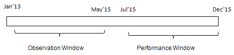
      R is one of the most popular programming language for performing statistical analysis and predictive modeling. Many recent surveys and studies claimed "R" holds a good percentage of market share in analytics industry. Data scientist role generally requires a candidate to know R/Python programming language. People who know R programming language are generally paid more than python and SAS programmers. In terms of advancement in R software, it has improved a lot in the recent years. It supports parallel computing and integration with big data technologies.
      R Interview Questions and Answers

      The following is a list of most frequently asked R Programming Interview Questions with detailed answer. It includes some basic, advanced or tricky questions related to R. Also it covers interview questions related to data science with R.


      1. How to determine data type of an object?

      class() is used to determine data type of an object. See the example below -
      x <- factor(1:5)
      class(x)
      It returns factor.
      Object Class
      To determine structure of an object, use str() function :
      str(x) returns "Factor w/ 5 level"

      Example 2 :
      xx <- data.frame(var1=c(1:5))
      class(xx)
      It returns "data.frame".
      str(xx) returns 'data.frame' : 5 obs. of  1 variable: $ var1: int

      2.  What is the use of mode() function?

      It returns the storage mode of an object.
      x <- factor(1:5)
      mode(x)
      The above mode function returns numeric.
      Mode Function
      x <- data.frame(var1=c(1:5))
      mode(x)
      It returns list.


      3. Which data structure is used to store categorical variables?

      R has a special data structure called "factor" to store categorical variables. It tells R that a variable is nominal or ordinal by making it a factor.
      gender = c(1,2,1,2,1,2)
      gender = factor(gender)
      gender
      4. How to check the frequency distribution of a categorical variable?

      The table function is used to calculate the count of each categories of a categorical variable.
      gender = factor(c("m","f","f","m","f","f"))
      table(gender)
      Output

      If you want to include % of values in each group, you can store the result in data frame using data.frame function and the calculate the column percent.
      t = data.frame(table(gender))
      t$percent= round(t$Freq / sum(t$Freq)*100,2)
      Frequency Distribution

      5.  How to check the cumulative frequency distribution of a categorical variable

      The cumsum function is used to calculate the cumulative sum of a categorical variable.
      gender = factor(c("m","f","f","m","f","f"))
      x = table(gender)
      cumsum(x)
      Cumulative Sum

      If you want to see the cumulative percentage of values, see the code below :
      t = data.frame(table(gender))
      t$cumfreq = cumsum(t$Freq)
      t$cumpercent= round(t$cumfreq / sum(t$Freq)*100,2)
      Cumulative Frequency Distribution


      6. How to produce histogram

      The hist function is used to produce the histogram of a variable.
      df = sample(1:100, 25)
      hist(df, right=FALSE)
      Produce Histogram with R
      To improve the layout of histogram, you can use the code below
      colors = c("red", "yellow", "green", "violet", "orange", "blue", "pink", "cyan")
      hist(df,  right=FALSE,  col=colors, main="Main Title ", xlab="X-Axis Title")
      7. How to produce bar graph

      First calculate the frequency distribution with table function and then apply barplot function to produce bar graph
      mydata = sample(LETTERS[1:5],16,replace = TRUE)
      mydata.count= table(mydata)
      barplot(mydata.count)
      To improve the layout of bar graph, you can use the code below:
      colors = c("red", "yellow", "green", "violet", "orange", "blue", "pink", "cyan")
      barplot(mydata.count, col=colors, main="Main Title ", xlab="X-Axis Title")
      Bar Graph with R

      8. How to produce Pie Chart

      First calculate the frequency distribution with table function and then apply pie function to produce pie chart.
      mydata = sample(LETTERS[1:5],16,replace = TRUE)
      mydata.count= table(mydata)
      pie(mydata.count, col=rainbow(12))
      Pie Chart with R

      9. Multiplication of 2 vectors having different length

      For example, you have two vectors as defined below -
      x <- c(4,5,6)
      y <- c(2,3)
      If you run this vector z <- x*y , what would be the output? What would be the length of z?

      It returns 8 15 12 with the warning message as shown below. The length of z is 3 as it has three elements.
      Multiplication of vectors


      First Step : It performs multiplication of the first element of vector x i.e. 4 with first element of vector y i.e. 2 and the result is 8. In the second step, it multiplies second element of vector x i.e. 5 with second element of vector b i.e. 3, and the result is 15. In the next step, R multiplies first element of smaller vector (y) with last element of bigger vector x. 

      Suppose the vector x would contain four elements as shown below :
      x <- c(4,5,6,7)
      y <- c(2,3)
      x*y
      It returns 8 15 12 21. It works like this : (4*2) (5*3) (6*2) (7*3)

      10. What are the different data structures R contain?

      R contains primarily the following data structures : 
      1. Vector
      2. Matrix
      3. Array
      4. List
      5. Data frame
      6. Factor
      The first three data types (vector, matrix, array) are homogeneous in behavior. It means all contents must be of the same type. The fourth and fifth data types (list, data frame) are heterogeneous in behavior. It implies they allow different types. And the factor data type is used to store categorical variable.


      11. How to combine data frames?

      Let's prepare 2 vectors for demonstration :
      x = c(1:5)
      y = c("m","f","f","m","f")
      The cbind() function is used to combine data frame by columns.
      z=cbind(x,y)
      cbind : Output

      The rbind() function is used to combine data frame by rows.
      z = rbind(x,y)
      rbind : Output

      While using cbind() function, make sure the number of rows must be equal in both the datasets. While using rbind() function, make sure both the number and names of columns must be same. If names of columns would not be same, wrong data would be appended to columns or records might go missing.

      12. How to combine data by rows when different number of columns?

      When the number of columns in datasets are not equal, rbind() function doesn't work to combine data by rows. For example, we have two data frames df and df2. The data frame df has 2 columns and df2 has only 1 variable. See the code below -
      df = data.frame(x = c(1:4), y = c("m","f","f","m"))
      df2 = data.frame(x = c(5:8))
      The bind_rows() function from dplyr package can be used to combine data frames when number of columns do not match.
      library(dplyr)
      combdf = bind_rows(df,df2)

      13.  What are valid variable names in R?

      A valid variable name consists of letters, numbers and the dot or underline characters. A variable name can start with either a letter or the dot followed by a character (not number).
      A variable name such as .1var is not valid. But .var1 is valid.
      A variable name cannot have reserved words. The reserved words are listed below -
      if else repeat while function for in next break
      TRUE FALSE NULL Inf NaN NA NA_integer_ NA_real_ NA_complex_ NA_character_
      A variable name can have maximum to 10,000 bytes.

      14. What is the use of with() and by() functions? What are its alternatives?

      Suppose you have a data frame as shown below -
      df=data.frame(x=c(1:6), y=c(1,2,4,6,8,12))
      You are asked to perform this calculation : (x+y) + (x-y) . Most of the R programmers write like code below -
      (df$x + df$y) + (df$x - df$y)
      Using with() function, you can refer your data frame and make the above code compact and simpler-
      with(df, (x+y) + (x-y))
      The with() function is equivalent to pipe operator in dplyr package. See the code below -
      library(dplyr)
      df %>% mutate((x+y) + (x-y))

      by() function in R

      The by() function is equivalent to group by function in SQL. It is used to perform calculation by a factor or a categorical variable. In the example below, we are computing mean of variable var2 by a factor var1.
      df = data.frame(var1=factor(c(1,2,1,2,1,2)), var2=c(10:15))
      with(df, by(df, var1, function(x) mean(x$var2)))
      The group_by() function in dply package can perform the same task.
      library(dplyr)
      df %>% group_by(var1)%>% summarise(mean(var2))

      15. How to rename a variable?

      In the example below, we are renaming variable var1 to variable1.
      df = data.frame(var1=c(1:5))
      colnames(df)[colnames(df) == 'var1'] <- 'variable1'
      The rename() function in dplyr package can also be used to rename a variable.
      library(dplyr)
      df= rename(df, variable1=var1)

      16. What is the use of which() function in R?

      The which() function returns the position of elements of a logical vector that are TRUE. In the example below, we are figuring out the row number wherein the maximum value of a variable x is recorded.
      mydata=data.frame(x = c(1,3,10,5,7))
      which(mydata$x==max(mydata$x))
      It returns 3 as 10 is the maximum value and it is at 3rd row in the variable x.


      17. How to calculate first non-missing value in variables?

      Suppose you have three variables X, Y and Z and you need to extract first non-missing value in each rows of these variables.
      data = read.table(text="
      X Y Z
      NA 1 5
      3 NA 2
      ", header=TRUE)
      The coalesce() function in dplyr package can be used to accomplish this task.
      library(dplyr)
      data %>% mutate(var=coalesce(X,Y,Z))
      COALESCE Function in R

      18. How to calculate max value for rows?

      Let's create a sample data frame
      dt1 = read.table(text="
      X Y Z
      7 NA 5
      2 4 5
      ", header=TRUE)
      With apply() function, we can tell R to apply the max function rowwise. The na,rm = TRUE is used to tell R to ignore missing values while calculating max value. If it is not used, it would return NA.
      dt1$var = apply(dt1,1, function(x) max(x,na.rm = TRUE)) 
      Output

      19. Count number of zeros in a row
      dt2 = read.table(text="
      A B C
      8 0 0
      6 0 5
      ", header=TRUE)
      apply(dt2,1, function(x) sum(x==0))

      20. Does the following code work?
      ifelse(df$var1==NA, 0,1)
      It does not work. The logic operation on NA returns NA. It does not TRUE or FALSE.

      This code works ifelse(is.na(df$var1), 0,1)


      21. What would be the final value of x after running the following program?

      x = 3
      mult <- function(j)
      {
        x = j * 2
        return(x)
      }

      mult(2)
      [1] 4

      Answer : The value of 'x' will remain 3. See the output shown in the image below-
      Output
      It is because x is defined outside function. If you want to change the value of x after running the function, you can use the following program:
      x = 3
      mult <- function(j)
      {
        x <<- j * 2
        return(x)
      }
      mult(2)
      x
      The operator "<<-" tells R to search in the parent environment for an existing definition of the variable we want to be assigned.

      22. How to convert a factor variable to numeric

      The as.numeric() function returns a vector of the levels of your factor and not the original values. Hence, it is required to convert a factor variable to character before converting it to numeric.
      a <- factor(c(5, 6, 7, 7, 5))
      a1 = as.numeric(as.character(a))
      23. How to concatenate two strings?

      The paste() function is used to join two strings. A single space is the default separator between two strings.
      a = "Deepanshu"
      b = "Bhalla"
      paste(a, b)
      It returns "Deepanshu Bhalla"

      If you want to change the default single space separator, you can add sep="," keyword to include comma as a separator.
      paste(a, b, sep=",") returns "Deepanshu,Bhalla"

      24. How to extract first 3 characters from a word

      The substr() function is used to extract strings in a character vector. The syntax of substr function is substr(character_vector, starting_position, end_position)
      x = "AXZ2016"
      substr(x,1,3)
      Character Functions Explained


      25. How to extract last name from full name

      The last name is the end string of the name. For example, Jhonson is the last name of "Dave,Jon,Jhonson".
      dt2 = read.table(text="
      var
      Sandy,Jones
      Dave,Jon,Jhonson
      ", header=TRUE)
      The word() function of stringr package is used to extract or scan word from a string. -1 in the second parameter  denotes the last word.
      library(stringr)
      dt2$var2 = word(dt2$var, -1, sep = ",")

      26. How to remove leading and trailing spaces

      The trimws() function is used to remove leading and trailing spaces.
      a = " David Banes "
      trimws(a)
      It returns "David Banes".

      27. How to generate random numbers between 1 and 100

      The runif() function is used to generate random numbers.
      rand = runif(100, min = 1, max = 100)

      28. How to apply LEFT JOIN in R?

      LEFT JOIN implies keeping all rows from the left table (data frame) with the matches rows from the right table. In the merge() function, all.x=TRUE denotes left join.
      df1=data.frame(ID=c(1:5), Score=runif(5,50,100))
      df2=data.frame(ID=c(3,5,7:9), Score2=runif(5,1,100))
      comb = merge(df1, df2, by ="ID", all.x = TRUE)
      Left Join (SQL Style)
      library(sqldf)
      comb = sqldf('select df1.*, df2.* from df1 left join df2 on df1.ID = df2.ID')

      Left Join with dply package 
      library(dplyr)
      comb = left_join(df1, df2, by = "ID")


      29. How to calculate cartesian product of two datasets

      The cartesian product implies cross product of two tables (data frames). For example, df1 has 5 rows and df2 has 5 rows. The combined table would contain 25 rows (5*5)
      comb = merge(df1,df2,by=NULL)
      CROSS JOIN (SQL Style)
      library(sqldf)
      comb2 = sqldf('select * from df1 join df2 ')

      30. Unique rows common to both the datasets

      First, create two sample data frames

      df1=data.frame(ID=c(1:5), Score=c(50:54))
      df2=data.frame(ID=c(3,5,7:9), Score=c(52,60:63))
      library(dplyr)
      comb = intersect(df1,df2)
      library(sqldf)
      comb2 = sqldf('select * from df1 intersect select * from df2 ')
      Output : Intersection with R

      31. How to measure execution time of a program in R?

      There are multiple ways to measure running time of code. Some frequently used methods are listed below -

      R Base Method
      start.time <- Sys.time()
      runif(5555,1,1000)
      end.time <- Sys.time()
      end.time - start.time
      With tictoc package
      library(tictoc)
      tic()
      runif(5555,1,1000)
      toc()

      32. Which package is generally used for fast data manipulation on large datasets?

      The package data.table performs fast data manipulation on large datasets. See the comparison between dplyr and data.table.

      # Load data
      library(nycflights13)
      data(flights)
      df = setDT(flights)

      # Load required packages
      library(tictoc)
      library(dplyr)
      library(data.table)

      # Using data.table package
      tic()
      df[arr_delay > 30 & dest == "IAH",
         .(avg = mean(arr_delay),
           size = .N),
         by = carrier]
      toc()

      # Using dplyr package
      tic()
      flights %>% filter(arr_delay > 30 & dest == "IAH") %>%
        group_by(carrier) %>% summarise(avg = mean(arr_delay), size = n())
      toc()

      Result : data.table package took 0.04 seconds. whereas dplyr package took 0.07 seconds. So, data.table is approx. 40% faster than dplyr. Since the dataset used in the example is of medium size, there is no noticeable difference between the two. As size of data grows, the difference of execution time gets bigger.

      33. How to read large CSV file in R?

      We can use fread() function of data.table package.
      library(data.table)
      yyy = fread("C:\\Users\\Dave\\Example.csv", header = TRUE)

      We can also use read.big.matrix() function of bigmemory package.

      34. What is the difference between the following two programs ?

      1. temp = data.frame(v1<-c(1:10),v2<-c(5:14))
      2. temp = data.frame(v1=c(1:10),v2=c(5:14))

      In the first case, it created two vectors v1 and v2 and a data frame temp which has 2 variables with improper variable names. The second code creates a data frame temp with proper variable names.

      35. How to remove all the objects
      rm(list=ls())

      36. What are the various sorting algorithms in R?

      Major five sorting algorithms :
      1. Bubble Sort
      2. Selection Sort
      3. Merge Sort
      4. Quick Sort
      5. Bucket Sort

      37. Sort data by multiple variables

      Create a sample data frame
      mydata = data.frame(score = ifelse(sign(rnorm(25))==-1,1,2),
                          experience= sample(1:25))
      Task : You need to sort score variable on ascending order and then sort experience variable on descending order.

      R Base Method
      mydata1 <- mydata[order(mydata$score, -mydata$experience),]
      With dplyr package
      library(dplyr)
      mydata1 = arrange(mydata, score, desc(experience))

      38. Drop Multiple Variables

      Suppose you need to remove 3 variables - x, y and z from data frame "mydata".

      R Base Method
      df = subset(mydata, select = -c(x,y,z))
      With dplyr package 
      library(dplyr)
      df = select(mydata, -c(x,y,z))

      40. How to save everything in R session
      save.image(file="dt.RData")

      41. How R handles missing values?

      Missing values are represented by capital NA.

      To create a new data without any missing value, you can use the code below :
      df <- na.omit(mydata)

      42. How to remove duplicate values by a column

      Suppose you have a data consisting of 25 records. You are asked to remove duplicates based on a column. In the example, we are eliminating duplicates by variable y.
      data = data.frame(y=sample(1:25, replace = TRUE), x=rnorm(25))
      R Base Method
      test = subset(data, !duplicated(data[,"y"]))
      dplyr Method 
      library(dplyr)
      test1 = distinct(data, y, .keep_all= TRUE)

      43. Which packages are used for transposing data with R

      The reshape2 and tidyr packages are most popular packages for reshaping data in R.

      Explanation : Transpose Data


      44. Calculate number of hours, days, weeks, months and years between 2 dates

      Let's set 2 dates :
      dates <- as.Date(c("2015-09-02", "2016-09-05"))
      difftime(dates[2], dates[1], units = "hours")
      difftime(dates[2], dates[1], units = "days")
      floor(difftime(dates[2], dates[1], units = "weeks"))
      floor(difftime(dates[2], dates[1], units = "days")/365)
      With lubridate package
      library(lubridate)
      interval(dates[1], dates[2]) %/% hours(1)
      interval(dates[1], dates[2]) %/% days(1)
      interval(dates[1], dates[2]) %/% weeks(1)
      interval(dates[1], dates[2]) %/% months(1)
      interval(dates[1], dates[2]) %/% years(1)
      The number of months unit is not included in the base difftime() function so we can use interval() function of lubridate() package.

      45. How to add 3 months to a date
      mydate <- as.Date("2015-09-02")
      mydate + months(3)

      46. Extract date and time from timestamp
      mydate <- as.POSIXlt("2015-09-27 12:02:14")
      library(lubridate)
      date(mydate) # Extracting date part
      format(mydate, format="%H:%M:%S") # Extracting time part
      Extracting various time periods
      day(mydate)
      month(mydate)
      year(mydate)
      hour(mydate)
      minute(mydate)
      second(mydate)

      47. What are various ways to write loop in R

      There are primarily three ways to write loop in R
      1. For Loop
      2. While Loop
      3. Apply Family of Functions such as Apply, Lapply, Sapply etc

      48. Difference between lapply and sapply in R

      lapply returns a list when we apply a function to each element of a data structure. whereas sapply returns a vector.

      49. Difference between sort(), rank() and order() functions?

      The sort() function is used to sort a 1 dimension vector or a single variable of data.
      The rank() function returns the ranking of each value.
      The order() function returns the indices that can be used to sort the data.

      Example :
      set.seed(1234)
      x = sample(1:50, 10)  
      x
      [1]  6 31 30 48 40 29  1 10 28 22

      sort(x)
      [1]  1  6 10 22 28 29 30 31 40 48

      It sorts the data on ascending order.

      rank(x)
      [1]  2  8  7 10  9  6  1  3  5  4

      2 implies the number in the first position is the second lowest and 8 implies the number in the second position is the eighth lowest.

      order(x)
       [1]  7  1  8 10  9  6  3  2  5  4

      7 implies the 7th value of x is the smallest value, so 7 is the first element of order(x) and i refers to the first value of x is the second smallest.
      If you run x[order(x)], it would give you the same result as sort() function. The difference between these two functions lies in two or more dimensions of data (two or more columns). In other words, the sort() function cannot be used for more than 1 dimension whereas x[order(x)] can be used.

      50.  Extracting Numeric Variables
      cols <- sapply(mydata, is.numeric)
      abc = mydata [,cols]

      Data Science with R Interview Questions

      The list below contains most frequently asked interview questions for a role of data scientist. Most of the roles related to data science or predictive modeling require candidate to be well conversant with R and know how to develop and validate predictive models with R.

      51. Which function is used for building linear regression model?

      The lm() function is used for fitting a linear regression model.


      52. How to add interaction in the linear regression model?

      :An interaction can be created using colon sign (:). For example, x1 and x2 are two predictors (independent variables). The interaction between the variables can be formed like x1:x2. 
      See the example below -
      linreg1 <- lm(y ~ x1 + x2 + x1:x2, data=mydata)
      The above code is equivalent to the following code :
      linreg1 <- lm(y ~ x1*x2, data=mydata)
      x1:x2 - It implies including both main effects (x1 + x2) and interaction (x1:x2).

      53. How to check autocorrelation assumption for linear regression?

      durbinWatsonTest() function

      54. Which function is useful for developing a binary logistic regression model?

      glm() function with family = "binomial"

      55. How to perform stepwise variable selection in logistic regression model?

      Run step() function after building logistic model with glm() function.

      56. How to do scoring in the logistic regression model?

      Run predict(logit_model, validation_data, type = "response")


      57. How to split data into training and validation?
      dt = sort(sample(nrow(mydata), nrow(mydata)*.7))
      train<-mydata[dt,]
      val<-mydata[-dt,]

      58. How to standardize variables?

      data2 = scale(data)

      59. How to validate cluster analysis

      Validate Cluster Analysis

      60. Which are the popular R packages for decision tree?

      rpart, party


      61. What is the difference between rpart and party package for developing a decision tree model?

      rpart is based on Gini Index which measures impurity in node. Whereas ctree() function from "party" package uses a significance test procedure in order to select variables.

      62. How to check correlation with R?

      cor() function

      63. Have you heard 'relaimpo' package? 

      It is used to measure the relative importance of independent variables in a model.

      64. How to fine tune random forest model?

      Use tuneRF() function

      65. What shrinkage defines in gradient boosting model?

      Shrinkage is used for reducing, or shrinking, the impact of each additional fitted base-learner (tree).


      66. How to make data stationary for ARIMA time series model?

      Use ndiffs() function which returns the number of difference required to make data stationary.

      67. How to automate arima model?

      Use auto.arima() function of forecast package

      68. How to fit proportional hazards model in R?

      Use coxph() function of survival package.

      69. Which package is used for market basket analysis?

      arules package

      70. Parallelizing Machine Learning Algorithms

      Link : Parallelizing Machine Learning

      Run R from SAS

      $
      0
      0
      This tutorial explains how to call or run R code from SAS environment. Both SAS and R are leaders in statistical analysis tools for analytics industry. Both the tools have its own advantages and disadvantages. Life would be very easy if we can integrate R with SAS. SAS officially made it possible to run R code via PROC IML. But PROC IML is a paid SAS module which causes user to incur additional cost. R comes with a strong list of machine learning / text mining packages and advanced graphic capabilities which makes it stand apart from SAS. For example, you are asked to forecast 5 years sales. In SAS, you have to purchase SAS ETS module for forecasting procedures such as Proc ARIMA, Proc Forecast etc. In R, forecasting package is available for free and more powerful than SAS forecasting procedures.
      Run R from SAS
      Xin Wei developed a macro called PROC_R which allows R language to be submitted with a SAS program in the base SAS environment. Check out the link for reference. It was designed similar to PROC SQL which lets users to write SQL queries on SAS datasets.

      Steps to integrate R with SAS

      Step 1 : Download Proc_R Code

      Step 2 : Save the file in desired location.

      Step 3 : Open the code and update the path of R executable file in the code below.
      %macro quit(rpath=%str(C:\Progra~1\R\R-3.3.1\bin\R.exe))
      Note : Make sure you use 'Progra~1' instead of 'Program Files' in the path. For example, my R executable file is saved in this path - C:\Program Files\R\R-3.3.1\bin\R.exe but i used this path - C:\Progra~1\R\R-3.3.1\bin\R.exe

      Step 4 : Open Base SAS and call proc_R macro. Replace the existing path in the code with your own path where you have saved proc_R code.
      %include "C:\Users\Deepanshu\Desktop\proc_R.sas";
      Step 5 : Run R inside SAS environment. See the SAS program below -
      %Proc_R(SAS2R=,R2SAS=);
      cards4;
      /********/
      /*R Code*/
      /********/
      ;;;;
      %quit;

      Proc_R Parameters

      1. SAS2R   - specifies the names of SAS datasets to be converted to R dataframe. Can be single file name or  multiple files whose names are separated by space.
      2. R2SAS   - specifies the names of R data frames to be converted to SAS datasets. Can be single file name or multiple files whose names are separated by space.

      Examples : Proc_R

      Create a sample data
      data example;
      input Srl x1-x5;
      cards;
      1 . 89 85 . 87
      2 79 73 74 . .
      3 80 82 . 85 .
      ;
      run;
      Example 1 : Calculating Summary Statistics

      The following program first exports input data in CSV format and R code. Then it imports CSV data from the working directory into R and run the code you put inside %proc_R. Later it exports R log, data frame and image which are later imported in SAS. Here, we are telling SAS to integrate with R to calculate summary statistics on example dataset.
      %include "C:\Users\Deepanshu\Desktop\proc_R.sas";

      /*Run Summary Statistics*/
      %Proc_R(SAS2R=example,R2SAS=);
      cards4;
      setwd("C:/Users/Deepanshu/Documents")
      summary(example)
      ;;;;
      %quit;

      proc print data=rlog;
      run;
      Note : It is required to set the working directory with setwd() function. Update your directory in the setwd() function.
      Summary displayed in SAS result window

      The output shown in the image above is a truncated one as the real output is large in size.

      Example 2 : Data Manipulation with dplyr Package

      In the program below, we are loading dplyr library and calculating first non-missing record in each row. The calculation would be done in R and later SAS exports dataframe df.
      %Proc_R(SAS2R=example,R2SAS=df);
      cards4;
      setwd("C:/Users/Deepanshu/Documents")
      library(dplyr)
      df = mutate(example,nonmiss=coalesce(x1,x2,x3,x4,x5))
      ;;;;
      %quit;

      Example3 : Creating Bar Chart

      The following code creates a bar chart in R and later displayed in SAS Results Viewer.
      %Proc_R(SAS2R=,R2SAS=);
      cards4;
      setwd("C:/Users/Deepanshu/Documents")
      mydata = sample(LETTERS[1:5],16,replace = TRUE)
      mydata.count= table(mydata)
      barplot(mydata.count)
      colors = c("red", "yellow", "green", "violet", "orange", "blue", "pink", "cyan")
      barplot(mydata.count, col=colors, main="Main Title ", xlab="X-Axis Title")
      ;;;;
      %quit;

      Example 4 : Build ARIMA Model in R
      data arimaexample;
      input sales @@;
      cards;
      360358357
      374371385
      385389398
      400412424
      418412408
      420424438
      435438446
      451456470
      457448440
      456457469
      473477483
      490498503
      ;
      run;
      %Proc_R(SAS2R=arimaexample,R2SAS=Forecastmodel);
      cards4;
      setwd("C:/Users/Deepanshu/Documents")
      library(forecast)

      # Convert it to ts object
      dat = data.frame(arimaexample)
      tsdata = ts(dat)

      # Plot time series data
      plot.ts(tsdata)
      tsdisplay(tsdata)

      # Box lambda Transformation
      lambda = BoxCox.lambda(tsdata)

      #lambda close to 1 means no transformation required
      tsdata2 = BoxCox(tsdata, lambda=lambda)
      plot.ts(tsdata2)

      # Unit Ratio Tests
      library(tseries)
      adf = adf.test(tsdata2)
      kpss = kpss.test(tsdata2)

      # Number of Difference Required to make data stationary
      ndiffs(tsdata2)
      tsdata3 = diff(tsdata2, differences = 1)
      final = auto.arima(tsdata, trace= TRUE, ic ="bic", approximation = FALSE, stepwise = FALSE)

      # predict the next 5 periods
      Forecastmodel = forecast.Arima(final, h = 5)

      ;;;;
      %quit;

      proc print data= rlog;
      run;

      Example 5 : Supports Multiple datasets / dataframes

      In the macro, we can also specify multiple SAS datasets or data frames. In the code below, we have specified multiple SAS datasets that would be imported into R and then perform some calculation and later multiple R data frames would be exported.
      %Proc_R(SAS2R=example arimaexample,R2SAS= df1 df2);
      cards4;
      setwd("C:/Users/Deepanshu/Documents")
      df1=data.frame(mean(as.numeric(arimaexample$sales)))
      df2=data.frame(sum(is.na(example)))
      ;;;;
      %quit;
      proc print data = df1;
      proc print data = df2;
      run;

      SAS : Advanced String Manipulation

      $
      0
      0
      This post covers how to deal some of the advanced string operations with SAS. In SAS, there are various functions available for handling character strings but sometimes they are not enough to manipulate character strings.

      Example 1 : Generate frequently used keywords

      Suppose you have a list of customer complaints with their open-ended comments You are asked to analyze it. The most common (or basic) text mining technique is to generate common used words in the list of complaints. It is easily possible via SAS text miner but a little bit complicated to be done via base SAS. The following SAS macro accomplish this task.
      %macro frequency(inputdata=,var=,outdata=);

      data test2;
      set &inputdata.;
      varr = compress(lowcase(&var.),'','ak');
      do i= 1 to countw(varr);
      var1= scan(varr,i);
      output;
      end;
      run;

      proc sql noprint;
      create table &outdata. as
      select var1, count(*) as N from test2
      where length(var1) > 2
      group by 1
      order by N desc;
      quit;
      %mend;

      %frequency(inputdata=temp,var=var,outdata=freqlist);
      Macro Parameters

      1. inputdata : Specify the name of the dataset in which open-ended comments exist
      2. var : Specify the name of the variable which contains comments
      3. outdata : Specify the name you want to assign to the output dataset
      SAS : Frequency of Words

      Areas of Improvement
      In the macro, this line of code "where length(var1) > 2" removes all keywords having length less than or equal to 2. It is to remove common non-meaningful words like "a", "an", "be", "is", "am""of""on""in" etc. It does not cover exhaustive list of non-meaningful keywords such as "the" ,"and", "that" etc. Also, this WHERE condition can remove important keywords that are abbreviations of some department / business unit etc. Example, CA refers to Corporate Agency. So, instead of using this line of code, prepare an exclusion list which can be used to exclude non-meaningful keywords.

      Example 2 : Reverse a Character String

      Suppose you have a list of words. You are asked to reverse it.

      Create a Sample Dataset
      data temp;
      input list $50.;
      cards;
      listendata
      saspythonr
      datascience
      analytics
      ;
      run;
       REVERSE Function
      data temp2;
      set temp;
      x = left(reverse(list));
      run;
      In SAS, there is a function available for reversing a string. The function is called REVERSE. The LEFT function is used before REVERSE function to remove leading spaces.
      SAS : Reverse String
      You may want to get your hands dirty by writing code for it without using REVERSE function. You can do it by extracting each letter from a string using DO LOOP and then reverse it with PROC SORT, RETAIN and FIRST., LAST. variables. See the code below -
      data test;
      set temp;
      do i= 1 to length(list);
      list1= substr(list,i,1);
      output;
      end;
      run;

      proc sort data = test;
      by list descending i ;
      run;

      data test2;
      set test(keep = list list1);
      retain list2;
      by list;
      if first.list then list2=trim(list1);
      else list2 = cats("",list2,list1);
      if last.list;
      keep list list2;
      run;

      Example 3 :  Extracting Alternate Letters from a String

      Suppose you are asked to pull alternate letters from a character string. The logic for it is similar to the REVERSE code. A few changes are : (1) To increment by 2 in loop instead of 1. (2) No sorting letters on descending order.

      SAS : Alternate Letters
      data test2;
      set temp;
      do i= 1 to length(list) by 2;
      list1= substr(list,i,1);
      output;
      end;
      run;

      proc sort data = test2;
      by list;
      run;

      data test3;
      set test2(keep= list list1);
      retain list2;
      by list;
      if first.list then list2=trim(list1);
      else list2 = cats("",list2,list1);
      if last.list;
      keep list list2;
      run; 

      Identify Terrorists with Predictive Modeling

      $
      0
      0
      This article reveals 'Till what extent Predictive Modeling can be used'. Predictive Modeling is a process which is used to build a model with the help of historical data to predict future behavior. In the process of predictive modeling, we use statistical and machine learning techniques. In this post, we will see how predictive modeling / data mining techniques can be used to identify terrorists.
      Identify Terrorists Attacks with Predictive Modeling
      Terrorists attacks are happening in every part of the world. Every day government announces a new terror alert. It has become priority of every government to eradicate terrorism from their country. Some countries have developed analytics-driven software to predict or forecast terrorists attacks. The software identifies patterns from the historical data and predicts terrorist activities.
      The Australian Security Agency designed a terror attack system that let their citizens a clearer idea of whether they should be alert or alarmed. It classifies threats into five levels – Not Expected, Possible, Probable, Expected and Certain.

      Likelihood of being a Terrorist

      US National Security Agency use a machine learning algorithm to assess each person's likelihood of being a terrorist. They used Pakistan's mobile network metadata of 55 million people to develop a model to identify terrorists.

      Background
      Around 4,000 people have been killed by drone strikes in Pakistan since 2004. According to leaked documents on The Intercept, these drone strikes happened based on results from the machine learning algorithm. The disastrous result is that the thousands of innocent people in Pakistan may have been mislabelled as terrorists by the algorithm.
      Data
      Target / Dependent Variable - Whether a person is terrorist or not
      Predictors / Independent Variable - 80 Variables. Some of the variables are listed below -
      Travel Patterns
      No. of visits to terrorist states
      Moved Permanently to terrorist states
      Overnight Trips
      Travel on particular day of the week
      Regular Visits to locations of Interest
      Travel Phrases
      Other Predictors
      Low use / income calls only
      Excessive SIM or Handset Swapping
      Frequent Detach / Power-Down
      Common Contacts
      User Location
      Pattern of Life
      Social Network
      Visits to airports

      Data Preparation
      Number of Events  :  Data from just seven known terrorists.
      Number of Non-Events : 100,000 users were selected at random

      Algorithm

      Random Forest was used as a machine learning algorithm. No much detail is specified in the NSA presentation file. Not sure whether they used stacking/blending ensemble learning algorithm.


      Model Results :

      1. 50% False Negative Rate. It refers to "50% actual terrorists but model incorrectly predicted them as "Non-Terrorists".

      2.0.18% False Positive Rate.  It refers to "0.18% innocents, but model incorrectly predicted as terrorists.
      A false positive rate of 0.18 percent across 55 million people would mean 99,000 innocents mislabelled as "terrorists"
      In marketing or credit risk models, 0.18% false positive rate is considered as an excellent score. But it is dangerous in the context of human lives. Even 0.01% false positive rate of 55 million population implies 5,500 innocent people potentially being misclassified as "terrorists" and killed.
      The highest rated target according to this machine learning was Ahmad Zaidan, Al-Jazeera's long-time bureau chief in Islamabad.

      Issue / Challenges related to this kind of model

      1. Event Rate : The main issue of the model is that they used a very few events (7 terrorists) to train the model. Machine learning algorithms require more events than classical statistical techniques. 
      2. Unstructured Data : Huge amount of data but unstructured
      3. Collaboration between Countries : Official data sharing security pact
      4. Implementation : It is very dangerous to implement the model and kill someone after blindly following results from the model.

      Several areas where we can leverage analytics to identify terrorists activities
      1. Identifying terrorist financing which provides funds for terrorists activities
      2. Profiling people who are educated but involved in terrorists activities.
      3. Correlating terrorist attacks with trends in geo-politics and money trails

      SAS : Find Variable with the Max or Min in a row

      $
      0
      0
      This tutorial demonstrates how to find a variable with the maximum or minimum value for each row (observation) in SAS. It's pretty straightforward to calculate max or min value but a little problematic to identify the variable name against the value.

      Let's create Sample Data
      data readin;
      input y1-y6;
      cards;
      11 55 59 35 25 87
      12 79 73 74 86 29
      13 80 95 77 25 74
      ;
      run;
      Find Variable Name Containing Max Value in a row
      data out;
      set readin;
      array values y1-y6;
      largest = max(of values[*]);
      index    = whichn(largest, of values[*]);
      name = vname(values[index]);
      proc print;
      run;
      Output

      Explanation :
      1. array values y1-y6 : Lists all the variables for calculating max value
      2. max() function calculates maximum value of all the variables listed in step 1 across rows
      3. whichn() function returns the column index number of the matching value. In this case, it is searching the maximum value across rows and returns the column position in the listed variables. For example, it returns 6 in row 1 as 87 is the maximum value in row 1 and it is placed at 6th column of y1-y6
      4. vname() function returns the variable name. In this case, it calculates variable name of the largest value.

      To Find Variable Name containing minimum value
      Use min() function instead of max() in the code above and the remaining code would be same.

      Find Top 3 Variables

      Suppose you are asked to identify top 3 variables across rows. You can use largest function in SAS.

      LARGEST Function : Syntax
      largest(k, variables)
      k : kth value you want (2 for the second largest value)
      data want;
         set readin;
         array values[*] y1-y6;
         array large[3];
         array names[3] $32;
         do i = 1 to dim(large);
            large[i] = largest(i,of values[*]);
            index    = whichn(large[i],of values[*]);
            names[i] = vname(values[index]);
         end;
         drop i index;
      proc print;
      run;
      SAS : LARGEST values

      Explanation :
      1. array values[*] y1-y6  -  Specify all the variables from which you want to calculate top 3 variables
      2. array large[3] - Top 3 large values
      3. array names[3] $32 - Names of top 3 variables
      4. do i = 1 to dim(large) - 3 iterations for calculating first, second and third largest values
      5. large[i] = largest(i,of values[*]) - largest value when i =1, second largest when i =2 and so on.
      6. index = whichn(large[i],of values[*]) : Column index for kth largest values
      7. names[i]    = vname(values[index]) :  Extract the variable name of the largest using largest index
      8. drop i index; : Dropping Irrelevant Variables

      Find Bottom 3 Variables
      Refer the code above and change largest() function to smallest() function.

      SAS SQL : Use Distinct in CASE WHEN

      $
      0
      0
      This tutorial explains how to ignore duplicates while specifying conditions / criteria in SQL queries. You must have used DISTINCT keyword to remove duplicates. It is frequently used with COUNT function to calculate number of unique cases.

      Example 1 :

      Suppose you have three variables, say, 'id', 'x' and 'y'. You need to calculate number of distinct "y" values when x is less than 30. See the snapshot of data below -

      Dummy Dataset : CASE WHEN

      Let's create dataset in SAS 
      data temp;
      input id x y ;
      cards;
      1 25 30
      1 28 30
      1 40 25
      2 23 54
      2 34 54
      2 35 56
      ;
      run;

      SAS : PROC SQL
      proc sql;
      select count(distinct y) as unique_y,
      count(distinct case when x < 30 then y else . end) as unique_criteria
      from temp;
      quit;
      Output
      Explanation :
      1. The above program computes number of distinct values in variable 'y' when values of variable "x" is less than 30.
      2. The keyword DISTINCT is used to remove or ignore duplicate records.
      3. In the dataset, there are in total 3 cases in variable 'y' when x < 30. Whereas distinct number of cases in variable 'y' is equal to 2.

      Example 2 : 

      Suppose you are asked to group values by ID and then calculate sum of distinct values of y when x < 30. If condition is not met, then sum of all values of y.
      proc sql;
      select id, sum(distinct y) as sum_unique,
      coalesce(sum(distinct case when x < 30 then y end),0) +
      coalesce(sum(case when x >= 30 then y end),0) as sum_unique_criteria

      from temp
      group by 1;
      quit;
      Output : Example 2

      Explanation :
      1. Since the DISTINCT keyword works on a complete record, we need to write conditions "x <30" and "x>=30" separately in CASE WHEN.
      2. The COALESCE function tells SAS to replace missing values with 0 and then sum the returned values of both the conditions. If we don't use COALESCE, it would return missing when any of the two values which we want to add contains missing/null.
      Example 3 :

      Suppose you are asked to group data by variable 'ID' and then calculate maximum value of variable 'Y' when x is less than 30. Otherwise take all the values. At last, sum the returned values of both the conditions.
      Example 3 : Case When
      data temp;
      input id x y ;
      cards;
      1 25 30
      1 28 27
      1 40 25
      2 23 54
      2 29 55
      2 34 56
      ;
      run;
      proc sql;
      select id,
      coalesce(max(case when x < 30 then y end),0) +
      coalesce(sum(case when x >= 30 then y end),0) as sum_unique_criteria
      from temp
      group by 1;
      quit;
      Example 4 :

      Suppose you need to pick the maximum value in variable Y when duplicates in variable "X" and then group data by variable "ID" and compute number of cases where Y=1.
      Example 4 : CASE WHEN with DISTINCT
      data temp;
      input id x y ;
      cards;
      1 1 1
      1 1 0
      1 2 1
      2 3 0
      2 4 1
      2 4 1
      ;
      run;
      proc sql;
      select a.id,
      count(distinct case when y > 0 then max_y else . end) as count_distinct
      from temp a left join (select x, max(ranuni(123) * y) as max_y from temp group by 1) b
      on a.x = b.x
      group by 1;
      quit;

      How it works :
      1. When X = 1, it picks the maximum value of variable Y i.e. 1 and sets Y =1. Then it groups data by variable "ID", it checks the number of cases in which Y is equal to one after removing duplicates in X=1 cases. So it returns 2.
      2. The RANUNI() function is used to generate random numbers between 0 and 1 without replacement.The number 123 that is enclosed in the ranuni function is called seed which produces the same random numbers when it is run next time.
      3. In this case, the RANUNI() function makes Y as unique identifier so that we can later count these unique cases.

      SAS : Second Non-Missing Value

      $
      0
      0
      This tutorial demonstrates how to get second or second last non-missing value across rows. In SAS, there is a function called COALESCE to extract first non-missing value in a row. So it is an easy job to fetch first or last non-missing value but tricky to pull second or second last non-missing value. It is mostly used to see the customer behavior over past 2-3 periods before the account gets closed.

      Let's start with the basics

      Example 1 : Extract First or Last Non-Missing Value

      Example : COALESCE Function
      Dummy Dataset
      data example;
      input Srl x1-x5;
      cards;
      1 . 89 85 . 87
      2 79 73 74 . .
      3 80 95 . 95 .
      ;
      run;
      data out;
      set example;
      first = coalesce(of x1-x5);
      last = coalesce(of x5-x1);
      proc print noobs;
      run;

      The coalesce(of x1-x5) would check first non-missing in variables starting from x1 to x5 across rows and returns the values in each rows. To get last value in a row, just reverse the order of variables. The coalesce(of x5-x1) would return first non-missing in variables x5, x4, x3, x2, x1. So, it would be indirectly last value as order of variables is opposite.


      Example 2 : Extract Second Non-Missing Value

      data out;
      set example;
      array value x1-x5;
      array nvalue(5) _temporary_;
      first = coalesce(of value(*));
      index = whichn(first, of value(*));
      do i = 1 to dim(value);
      if i = index then nvalue(i) = .;
      else nvalue(i)= value(i);
      end;
      drop i index;
      second = coalesce(of nvalue(*));
      proc print noobs;
      run;
      Get Second Non-Missing Value
      How it works -
      1. First, create an array for variables from which we want to extract second non-missing value
      2. The idea is to make first non-missing value missing so that we can pull second non-missing value
      3. First, we need to create a temporary array of 5 variables in which we can store value.
      4. The function WHICHN is used to find the column position of first non-missing value. For example, it returns 2 for row 1 values.
      5. The DO LOOP is used to run the above steps iteratively in loop.

      Example 3 : Pull Second Last Non-Missing Value

      data out2;
      set example;
      array value x5-x1;
      array nvalue(5) _temporary_;
      last = coalesce(of value(*));
      index = whichn(last, of value(*));
      do i = 1 to dim(value);
      if i = index then nvalue(i) = .;
      else nvalue(i)= value(i);
      end;
      drop i index;
      secondlast = coalesce(of nvalue(*));
      proc print noobs;
      run;
      SAS : Second Last Non-Missing
      The only difference between second and third example is how variables are defined in array 'value'. In the example 3, we have reversed the position of variables to fetch second last non-missing value.

      Create Charts with SAS

      $
      0
      0
      This tutorial covers various techniques to modify and create charts or graphs with SAS. SAS has never been the first choice of analysts for creating graphs/charts as it requires time and skill to code the custom graphs in SAS. Analysts prefer MS Excel over SAS for creating graphs as it's a very quick and easy process in Excel. In this post, i would provide the clear explanation of how to make charts quickly with SAS.

      Prepare Dataset for Charts

      We would be using SASHELP.CLASS dataset for demonstration of bar charts. This dataset contains five variables such as Name, Sex, Age, Height and Weight for 19 students. I have picked 4 records from each of the two categories of sex MALE and FEMALE to make the dataset smaller so that graphs do not look TOO BIG in the post. Run the program below -
      proc rank data = sashelp.class descending out=temp (where=(weight_r <= 4));
      by sex;
      var weight;
      ranks weight_r;
      run;
      The above program would create a dataset called TEMP in WORK library which would contain only 8 rows / observations.

      Simple Horizontal Bar Chart

      Bar chart is one of the most commonly used charts. It's used to show comparison between two or more categories. It's applicable or acceptable in almost all the domains from BFSI to telecom.

      In the program below, HBAR represents horizontal bar, type = defines the type of statistics we need to compute. SUMVAR refers to summary variable. It does not imply SUM/ Addition.
      title1 "Weights of Students";
      proc gchart data=temp;
      hbar name / type=sum sumvar=weight;
      run;
      Bar Charts - Example 1

      Simple Vertical Bar Chart

      In this section, we are creating vertical bar chart. The only difference between the previous graph and this graph would be to change the option HBAR to VBAR.
      title1 "Weights of Students";
      proc gchart data=temp;
      vbar name / type=sum sumvar=weight;
      run;
      Vertical Bar Chart

      Add Labels in the Vertical Bar Chart

      The OUTSIDE= tells SAS to show specific statistics in the data label. In this case, it is SUM. It works only with VBAR option.
      title1 "Weights of Students";
      proc gchart data=temp;
      vbar name / type=sum sumvar=weight outside=sum;
      run;
      SAS Graphs : Adding Data Labels
      Note : You can use INSIDE= option to show data label at the end of the bars.

      Sort Bars

      You can use DESCENDING / ASCENDING option to sort the bars by their length.
      title1 "Weights of Students";
      proc gchart data=temp;
      vbar name / type=sum sumvar=weight descending outside=sum;
      run;
      SAS : Sort Bars

      Add / Remove Axes Title

      There are three axes to format in SAS.
      1. Midpoint (Use MAXIS option)
      2. Group (Use GAXIS option)
      3. Response (Use RAXIS option)
      In the following code, we are removing label from the X Axis and adding custom label in Y axis. The goptions htext=13pt htitle=15pt refers to the font size of the default text and chart title.
      title1 "Total Weights of Students";
      goptions htext=13pt htitle=15pt;
      axis1 label=none;
      axis2 label=('Weight in Pounds');

      proc gchart data=temp;
      vbar name / type=sum sumvar=weight descending
      maxis=axis1 raxis=axis2;
      run;
      quit;
      Add Axes Title

      Change Width of the Chart
      You can use WIDTH= option to increase width of the chart. It is very useful technique when we have a smaller number of categories. It is shown in the next section where we have only two categories.

      Mean Chart

      Suppose you are asked to create a chart which shows the comparison of weights of male vs female. The type=mean option is used to generate mean statistics of the two categories of variable SEX.
      title1 "Average Male vs. Female Weights";
      goptions htext=13pt htitle=15pt;
      axis1 label=none  value=(f="Arial/Bold""Female""Male"); ;
      axis2 label=(a=90 f="Arial/Bold"'Mean Weight in Pounds') order=(0 to 150 by 25) minor=none  offset=(0,0);
      proc gchart data=temp;
      vbar sex / width= 25 type=mean sumvar=weight descending
      maxis=axis1 raxis=axis2 outside=mean;
      run;
      quit;

      Mean Chart
      In this chart, we have done a lot of formatting. The detailed formatting tips are listed below -

      1. Assign Value Labels 'Male''Female' to X-axis. It is done via axis1 value = option.
      2. Change the orientation of Y-axis title with 'a=90' in axis2 label.
      3. Change the scale of Y axis with 'order=(0 to 150 by 25)'.
      4. minor=none turns off minor tick marks.
      5. offset=(0,0) remove space between the last number in the axis and the frame.

      Change color of the Chart

      You can set the color of the chart with PATTERN statement. The outline color of the bar can be changed with COUTLINE= option. We can also custom (hex) colors in the graph. See the custom color used in the following graph.
      pattern1 v=solid color=red;
      proc gchart data=temp;
      vbar sex / width= 25 type=mean sumvar=weight descending
      maxis=axis1 raxis=axis2 outside=mean coutline=gray;
      run;
      quit;

      Set Multiple Colors

      You can use multiple PATTERN statements with SUBGROUP= option to fill multiple colors in the graphs.
      title1 "Average Male vs. Female Weights";
      pattern1 value=solid color=pink;
      pattern2 value=solid color=cx42C0FB;
      proc gchart data=temp;
      vbar sex / width= 25 type=mean sumvar=weight descending
      maxis=axis1 raxis=axis2 outside=mean coutline=gray subgroup=sex;
      run;
      quit;
      SAS Graphs : Multiple Colors

      Percentage Chart
      Suppose you need to show the percentage of male and female students in a graph (including the count number).
      SAS : Percentage Chart
      title1 "% of Male vs. Female Students";
      goptions htext=13pt htitle=15pt;
      axis1 label=none  value=(f="Arial/Bold""Female""Male"); ;
      axis2 label=(a=90 f="Arial/Bold"'Percentage of Students') minor=none  offset=(0,0);
      proc gchart data=temp;
      vbar sex / width= 25 type=pct descending
      maxis=axis1 raxis=axis2 inside= freq outside=pct;
      run;
      quit;
      To show both frequent and %, use INSIDE= and OUTSIDE= options.

      Grouped Bar Chart

      You can use GROUP= option to create hierarchical / grouped bar chart in SAS.
      title;
      axis1 label=('MSRP') minor=none offset=(0,0);
      axis2 label=none;
      axis3 label=none offset=(7,7);
      proc gchart data=sashelp.cars;
      vbar type  / discrete type=mean sumvar=msrp
      group=origin coutline=gray raxis=axis1 maxis=axis2 gaxis=axis3 noframe;
      run;
      quit;
      SAS : Grouped Bar Chart

      Stacked Bar Chart

      The DISCRETE option is used to show each data value in a separate bar. The SUBGROUP= option tells SAS to fill different color in each of the groups.
      title;
      axis1 label=('MSRP') minor=none offset=(0,0);
      axis2 label=none offset=(7,7);
      proc gchart data=sashelp.cars;
      vbar type / discrete type=mean sumvar=msrp
      subgroup=origin coutline=gray width=10
      raxis=axis1 maxis=axis2 noframe;
      run;
      quit;

      SAS : Stacked Bar Chart

      Histogram

      Histogram is used to show distribution of continuous values in a graph. The LEVELS=4 implies we need to show only 4 bars in the histogram.
      title;
      goptions htext=10pt htitle=12pt;
      proc gchart data=temp;
      vbar weight / space=1 width=10 outside=freq levels=4 range;
      run; quit;

      Scatterplot

      Scatterplot is used to see the relationship between two variables. In the graph below, we are looking for relationship between height and weight by male and female.
      Scatterplot with SAS
      symbol1 value=circle height=3 interpol=none color=blue;
      symbol2 value=circle height=3 interpol=none color=red;
      proc gplot data=temp;
      plot height*weight=sex;
      run;
      PROC GPLOT is used to create scatter plot, box plot and line chart in SAS.

      Box Plot

      The following graph is a special case of Box plot in which we are displaying the distribution of continuous variable (height) by a categorical variable (sex).
      Box Plot
      title "Height Distribution by Sex";
      symbol1 value=circle height=3 interpol=none color=blue;
      axis1 minor=none offset=(0,0);
      axis2 offset=(20,20);
      proc gplot data=temp;
      plot height*sex=1 /
      vaxis=axis1 haxis=axis2 noframe;
      run;
      To show 25th, 50th and 75th percentile in the box-plot, use the code below. The only change in the code is to modify the symbol statement.
      title "Height Distribution by Sex";
      symbol1 interpol=boxt bwidth=4 color=blue;
      axis1 minor=none offset=(0,0);
      axis2 offset=(20,20);
      proc gplot data=temp;
      plot height*sex=1 /
      vaxis=axis1 haxis=axis2 noframe;
      run;
      Line Chart

      Line chart is used to show trends in data over some time periods.
      Line Chart with SAS
      title "Line Chart";
      symbol1 value=none interpol=sm color=blue;
      proc gplot data=sashelp.failure;
      where cause ="Contamination" and Process = "Process A";
      plot count*day;
      run;
      quit;
      The INTERPOL=SM in SYMBOL statement tells SAS to connect the dots/arrows and create a line.

      Data.Table Tutorial (with 50 Examples)

      $
      0
      0
      This tutorial describes how to manipulate data with data.table R package. It is considered as the fastest R package for data wrangling. Analysts generally call R programming not compatible with big datasets ( > 10 GB) as it is not memory efficient and loads everything into RAM. To change their perception, 'data.table' package comes into play. This package was designed to be concise and painless. There are many benchmarks done in the past to compare dplyr vs data.table. In every benchmark, data.table wins. The efficiency of this package was also compared with python' package (panda). And data.table wins. In CRAN, there are more than 200 packages that are dependent on data.table which makes it listed in the top 5 R's package. This post includes various examples and practice questions to make you familiar with the package.

      data.table Tutorial

      data.table Syntax

      The syntax of data.table is shown in the image below :
      data.table Syntax

      DT[ i , j , by]
      1. The first parameter of data.table i refers to rows. It implies subsetting rows. It is equivalent to WHERE clause in SQL
      2. The second parameter of data.table j refers to columns. It implies subsetting columns (dropping / keeping). It is equivalent to SELECT clause in SQL.
      3. The third parameter of data.table by refers to adding a group so that all calculations would be done within a group. Equivalent to SQL's GROUP BY clause.

      The data.table syntax is NOT RESTRICTED to only 3 parameters. There are other arguments that can be added to data.table syntax. The list is as follows -
      1. with, which
      2. allow.cartesian
      3. roll, rollends
      4. .SD, .SDcols
      5. on, mult, nomatch
      The above arguments would be explained in the latter part of the post.

      How to Install and load data.table Package
      install.packages("data.table") 
      #load required library
      library(data.table)

      Read Data

      In data.table package, fread() function is available to read or get data from your computer or from a web page. It is equivalent to read.csv() function of base R.
      mydata = fread("https://github.com/arunsrinivasan/satrdays-workshop/raw/master/flights_2014.csv")

      Describe Data

      This dataset contains 253K observations and 17 columns. It constitutes information about flights' arrival or departure time, delays, flight cancellation and destination in year 2014.
      nrow(mydata)
      [1] 253316
      ncol(mydata)
      [1] 17
      names(mydata)
       [1] "year"     "month"    "day"      "dep_time" "dep_delay""arr_time" "arr_delay"
       [8] "cancelled""carrier"  "tailnum"  "flight"   "origin"   "dest"     "air_time"
      [15] "distance" "hour"     "min"     
      head(mydata)
         year month day dep_time dep_delay arr_time arr_delay cancelled carrier tailnum flight
      1: 2014     1   1      914        14     1238        13         0      AA  N338AA      1
      2: 2014     1   1     1157        -3     1523        13         0      AA  N335AA      3
      3: 2014     1   1     1902         2     2224         9         0      AA  N327AA     21
      4: 2014     1   1      722        -8     1014       -26         0      AA  N3EHAA     29
      5: 2014     1   1     1347         2     1706         1         0      AA  N319AA    117
      6: 2014     1   1     1824         4     2145         0         0      AA  N3DEAA    119
         origin dest air_time distance hour min
      1:    JFK  LAX      359     2475    9  14
      2:    JFK  LAX      363     2475   11  57
      3:    JFK  LAX      351     2475   19   2
      4:    LGA  PBI      157     1035    7  22
      5:    JFK  LAX      350     2475   13  47
      6:    EWR  LAX      339     2454   18  24


      Selecting or Keeping Columns

      Suppose you need to select only 'origin' column. You can use the code below -
      dat1 = mydata[ , origin] # returns a vector
      The above line of code returns a vector not data.table.

      To get result in data.table format, run the code below :
      dat1 = mydata[ , .(origin)] # returns a data.table
      It can also be written like data.frame way
      dat1 = mydata[, c("origin"), with=FALSE]

      Keeping a column based on column position
      dat2 =mydata[, 2, with=FALSE]
      In this code, we are selecting second column from mydata.

      Keeping Multiple Columns

      The following code tells R to select 'origin', 'year', 'month', 'hour' columns.
      dat3 = mydata[, .(origin, year, month, hour)]

      Keeping multiple columns based on column position

      You can keep second through fourth columns using the code below -
      dat4 = mydata[, c(2:4), with=FALSE]

      Dropping a Column

      Suppose you want to include all the variables except one column, say. 'origin'. It can be easily done by adding ! sign (implies negation in R)
      dat5 = mydata[, !c("origin"), with=FALSE]

      Dropping Multiple Columns
      dat6 = mydata[, !c("origin", "year", "month"), with=FALSE]

      Keeping variables that contain 'dep'

      You can use %like% operator to find pattern. It is same as base R's grepl() functionSQL's LIKE operator and SAS's CONTAINS function.
      dat7 = mydata[,names(mydata) %like%"dep", with=FALSE]

      Rename Variables

      You can rename variables with setnames() function. In the following code, we are renaming a variable 'dest' to 'destination'.
      setnames(mydata, c("dest"), c("Destination"))
      To rename multiple variables, you can simply add variables in both the sides.
      setnames(mydata, c("dest","origin"), c("Destination", "origin.of.flight"))

      Subsetting Rows / Filtering

      Suppose you are asked to find all the flights whose origin is 'JFK'.
      # Filter based on one variable
      dat8 = mydata[origin == "JFK"]
      Select Multiple Values

      Filter all the flights whose origin is either 'JFK' or 'LGA'
      dat9 = mydata[origin %in% c("JFK", "LGA")]

      Apply Logical Operator : NOT

      The following program selects all the flights whose origin is not equal to 'JFK' and 'LGA'
      # Exclude Values
      dat10 = mydata[!origin %in% c("JFK", "LGA")]

      Filter based on Multiple variables

      If you need to select all the flights whose origin is equal to 'JFK' and carrier = 'AA'
      dat11 = mydata[origin == "JFK"& carrier == "AA"]

      Faster Data Manipulation with Indexing

      data.table uses binary search algorithm that makes data manipulation faster.

      Binary Search Algorithm
      Binary search is an efficient algorithm for finding a value from a sorted list of values. It involves repeatedly splitting in half the portion of the list that contains values, until you found the value that you were searching for.
      Suppose you have the following values in a variable :
      5, 10, 7, 20, 3, 13, 26
      You are searching the value 20 in the above list. See how binary search algorithm works -

      1. First, we sort the values 
      2. We would calculate the middle value i.e. 10.
      3. We would check whether 20 = 10? No. 20 < 10.
      4. Since 20 is greater than 10, it should be somewhere after 10. So we can ignore all the values that are lower than or equal to 10.
      5. We are left with 13, 20, 26. The middle value is 20. 
      6. We would again check whether 20=20. Yes. the match found.

      If we do not use this algorithm, we would have to search 5 in the whole list of seven values.

      It is important to set key in your dataset which tells system that data is sorted by the key column. For example, you have employee’s name, address, salary, designation, department, employee ID. We can use 'employee ID' as a key to search a particular employee.

      Set Key

      In this case, we are setting 'origin' as a key in the dataset mydata.
      # Indexing (Set Keys)
      setkey(mydata, origin)
      Note : It makes the data table sorted by the column 'origin'.

      How to filter when key is turned on.

      You don't need to refer the key column when you apply filter.
      data12 = mydata[c("JFK", "LGA")]

      Performance Comparison

      You can compare performance of the filtering process (With or Without KEY).
      system.time(mydata[origin %in% c("JFK", "LGA")])
      system.time(mydata[c("JFK", "LGA")])
      Performance - With or without KEY
      If you look at the real time in the image above, setting key makes filtering twice as faster than without using keys.

      Indexing Multiple Columns

      We can also set keys to multiple columns like we did below to columns 'origin' and 'dest'. See the example below.
      setkey(mydata, origin, dest)
      Filtering while setting keys on Multiple Columns
      # First key column 'origin' matches “JFK” and second key column 'dest' matches “MIA”
      mydata[.("JFK", "MIA")]
      It is equivalent to the following code :
      mydata[origin == "JFK"& dest == "MIA"]
      To identify the column(s) indexed by
      key(mydata)
      Result : It returns origin and dest as these are columns that are set keys.

      Sorting Data

      We can sort data using setorder() function, By default, it sorts data on ascending order.
      mydata01 = setorder(mydata, origin)

      Sorting Data on descending order

      In this case, we are sorting data by 'origin' variable on descending order.
      mydata02 = setorder(mydata, -origin)

      Sorting Data based on multiple variables

      In this example, we tells R to reorder data first by origin on ascending order and then variable 'carrier'on descending order.
      mydata03 = setorder(mydata, origin, -carrier)

      Adding Columns (Calculation on rows)

      You can do any operation on rows by adding := operator. In this example, we are subtracting 'dep_delay' variable from 'dep_time' variable to compute scheduled departure time.
      mydata[, dep_sch:=dep_time - dep_delay]

      Adding Multiple Columns

      mydata002 = mydata[, c("dep_sch","arr_sch"):=list(dep_time - dep_delay, arr_time - arr_delay)]

      IF THEN ELSE

      The 'IF THEN ELSE' conditions are very popular for recoding values. In data.table package, it can be done with the following methods :

      Method I :    mydata[, flag:= 1*(min < 50)]
      Method II :   mydata[, flag:= ifelse(min < 50, 1,0)]

      It means to set flag= 1 if min is less than 50. Otherwise, set flag =0.

      How to write Sub Queries (like SQL)

      We can use this format - DT[ ] [ ] [ ] to build a chain in data.table. It is like sub-queries like SQL.
      mydata[, dep_sch:=dep_time - dep_delay][,.(dep_time,dep_delay,dep_sch)]
      First, we are computing scheduled departure time and then selecting only relevant columns.


      Summarize or Aggregate Columns

      Like SAS PROC MEANS procedure, we can generate summary statistics of specific variables. In this case, we are calculating mean, median, minimum and maximum value of variable arr_delay.
      mydata[, .(mean = mean(arr_delay, na.rm = TRUE),
      median = median(arr_delay, na.rm = TRUE),
      min = min(arr_delay, na.rm = TRUE),
      max = max(arr_delay, na.rm = TRUE))]
      Summarize with data.table package
      Summarize Multiple Columns

      To summarize multiple variables, we can simply write all the summary statistics function in a bracket. See the command below-
      mydata[, .(mean(arr_delay), mean(dep_delay))]
      If you need to calculate summary statistics for a larger list of variables, you can use .SD and .SDcols operators. The .SD operator implies 'Subset of Data'. 
      mydata[, lapply(.SD, mean), .SDcols = c("arr_delay", "dep_delay")]
      In this case, we are calculating mean of two variables - arr_delay and dep_delay.

      Summarize all numeric Columns

      By default, .SD takes all continuous variables (excluding grouping variables)
      mydata[, lapply(.SD, mean)]

      Summarize with multiple statistics
      mydata[, sapply(.SD, function(x) c(mean=mean(x), median=median(x)))]


      GROUP BY (Within Group Calculation)

      Summarize by group 'origin
      mydata[, .(mean_arr_delay = mean(arr_delay, na.rm = TRUE)), by = origin]
      Summary by group

      Use key column in a by operation

      Instead of 'by', you can use keyby= operator.
      mydata[, .(mean_arr_delay = mean(arr_delay, na.rm = TRUE)), keyby = origin]

      Summarize multiple variables by group 'origin'
      mydata[, .(mean(arr_delay, na.rm = TRUE), mean(dep_delay, na.rm = TRUE)), by = origin]
       Or it can be written like below -
      mydata[, lapply(.SD, mean, na.rm = TRUE), .SDcols = c("arr_delay", "dep_delay"), by = origin]

      Remove Duplicates

      You can remove non-unique / duplicate cases with unique() function. Suppose you want to eliminate duplicates based on a variable, say. carrier.
      setkey(mydata, "carrier")
      unique(mydata)

      Suppose you want to remove duplicated based on all the variables. You can use the command below -
      setkey(mydata, NULL)
      unique(mydata)
      Note : Setting key to NULL is not required if no key is already set.

      Extract values within a group

      The following command selects first and second values from a categorical variable carrier.
      mydata[, .SD[1:2], by=carrier]

      Select LAST value from a group
      mydata[, .SD[.N], by=carrier]

      SQL's RANK OVER PARTITION

      In SQL, Window functions are very useful for solving complex data problems. RANK OVER PARTITION is the most popular window function. It can be easily translated in data.table with the help of frank() function. frank() is similar to base R's rank() function but much faster. See the code below.
      dt = mydata[, rank:=frank(-distance,ties.method = "min"), by=carrier]
      In this case, we are calculating rank of variable 'distance' by 'carrier'. We are assigning rank 1 to the highest value of 'distance' within unique values of 'carrier'.


      Cumulative SUM by GROUP

      We can calculate cumulative sum by using cumsum() function.
      dat = mydata[, cum:=cumsum(distance), by=carrier]

      Lag and Lead

      The lag and lead of a variable can be calculated with shift() function. The syntax of shift() function is as follows - shift(variable_name, number_of_lags, type=c("lag", "lead"))
      DT <- data.table(A=1:5)
      DT[ , X := shift(A, 1, type="lag")]
      DT[ , Y := shift(A, 1, type="lead")]
      Lag and Lead Function

      Between and LIKE Operator

      We can use %between% operator to define a range. It is inclusive of the values of both the ends.
      DT = data.table(x=6:10)
      DT[x %between% c(7,9)]
      The %like% is mainly used to find all the values that matches a pattern.
      DT = data.table(Name=c("dep_time","dep_delay","arrival"), ID=c(2,3,4))
      DT[Name %like%"dep"] 

      Merging / Joins

      The merging in data.table is very similar to base R merge() function. The only difference is data.table by default takes common key variable as a primary key to merge two datasets. Whereas, data.frame takes common variable name as a primary key to merge the datasets.

      Sample Data
      (dt1 <- data.table(A = letters[rep(1:3, 2)], X = 1:6, key = "A"))
      (dt2 <- data.table(A = letters[rep(2:4, 2)], Y = 6:1, key = "A"))
      Inner Join

      It returns all the matching observations in both the datasets.
      merge(dt1, dt2, by="A")

      Left Join

      It returns all observations from the left dataset and the matched observations from the right dataset.
      merge(dt1, dt2, by="A", all.x = TRUE)

      Right Join

      It returns all observations from the right dataset and the matched observations from the left dataset.
      merge(dt1, dt2, by="A", all.y = TRUE)

      Full Join

      It return all rows when there is a match in one of the datasets.
      merge(dt1, dt2, all=TRUE)


      Convert a data.table to data.frame

      You can use setDF() function to accomplish this task.
      setDF(mydata)
      Similarly, you can use setDT() function to convert data frame to data table.
      set.seed(123)
      X = data.frame(A=sample(3, 10, TRUE),
                     B=sample(letters[1:3], 10, TRUE)
      setDT(X, key = "A")

      Other Useful Functions

      Reshape Data
      It includes several useful functions which makes data cleaning easy and smooth. To reshape or transpose data, you can use dcast.data.table() and melt.data.table() functions. These functions are sourced from reshape2 package and make them efficient. It also add some new features in these functions.

      Rolling Joins
      It supports rolling joins. They are commonly used for analyzing time series data. A very R packages supports these kind of joins.

      Examples for Practise

      Q1. Calculate total number of rows by month and then sort on descending order
      mydata[, .N, by = month] [order(-N)]
      The .N operator is used to find count.

      Q2. Find top 3 months with high mean arrival delay
      mydata[, .(mean_arr_delay = mean(arr_delay, na.rm = TRUE)), by = month][order(-mean_arr_delay)][1:3]

      Q3. Find origin of flights having average total delay is greater than 20 minutes
      mydata[, lapply(.SD, mean, na.rm = TRUE), .SDcols = c("arr_delay", "dep_delay"), by = origin][(arr_delay + dep_delay) > 20]

      Q4.  Extract average of arrival and departure delays for carrier == 'DL' by 'origin' and 'dest' variables
      mydata[carrier == "DL",
              lapply(.SD, mean, na.rm = TRUE),
              by = .(origin, dest),
              .SDcols = c("arr_delay", "dep_delay")]

      Q5. Pull first value of 'air_time' by 'origin' and then sum the returned values when it is greater than 300
      mydata[, .SD[1], .SDcols="air_time", by=origin][air_time > 300, sum(air_time)]

      Endnotes

      This package provides a one-stop solution for data wrangling in R. It offers two main benefits - less coding and lower computing time. However, it's not a first choice of some of R programmers. Some prefer dplyr package for its simplicity. I would recommend learn both the packages. Check out dplyr tutorial. If you are working on data having size less than 1 GB, you can use dplyr package. It offers decent speed but slower than data.table package.

      Speed up SAS Code with Index

      $
      0
      0
      This tutorial demonstrates how to speed up SAS code with Indexes.
      SAS Index

      What is Index?

      Indexes are not something technical or related to SAS programming. It is something we use everyday to make our life easy. For example, every employee in an organization has an employee ID which is unique. It's easy for HR /Admin team to find information about a particular employee. First Name or Last Name of employees are not unique so it's better to record information by unique ID. So, employee information is indexed by employee ID. Let's take few more examples - dictionary is alphabetically sorted. So alphabets are index in this case. There can be multiple indexes to find information. For example, books in a library are sorted by topics (Science) and sub-topics (Physics /Chemistry / Bio / Statistics).

      In SAS, Index is used to store observations in an ascending order and later access them quickly from a variable. In simple words, it minimizes some steps of searching a particular value by telling SAS the nearest /exact location of the value you are searching for. Confused? Read the next section.

      How Index works?

      When Index is used, SAS runs a binary search algorithm on the data set.

      Binary search is a performance improvement algorithm for searching a particular observation from a sorted variable. It works by continuously dividing in half of the total number of observations and search the value in the half of the list, until you got the value that you were looking for.

      Example


      Let's assume you have a variable CustomerID :
      15, 20, 3, 16, 9, 17, 13
      You are finding the information of customer having CustomerID equals to 17. See the steps below to find the value -
      1. First, sort the CustomerID variable. We will have these values - {3,9,13,15,16,17,20}
      2. Calculate the median (middle value) of the list i.e. 15.
      3. We would check whether search_value = median? Is 17 =15? No. 17 > 15.
      4. Ignore all the values that are less than or equal to 15 as 17 is a higher number than 15.
      5. Now, we need to search in the remaining list i.e. 16, 17, 20. The middle value is 17.
      6. Is 17 = 17? Yes. the value found.
      If you do not create an index SAS would search 17 sequentially in the whole list. The above is a simple example of a few values. If you have millions of observations, it would take a hell lot of time to search a particular value sequentially in the variable.

      When to Use Index ?

      1. Size of Subset Records

      You should only use Index if you need to pull a small subset from a large SAS data set. See the definition of 'small' and 'large' in the table below -
      Subset SizeWill Indexing Improve?
      1% - 15%Definitely
      16% - 20%Probably
      21% - 33%Might Improve or Worse
      34% - 100%Not Improve

      2. Variable Consideration

      It is recommended to index only those variables that have a high number of distinct values. For example, Customer ID as it is unique at customer level so it would have a high number of unique records.  But the variable 'sex' would have only two distinct values so it would not be a good choice to index.


      3. Usage Level

      If you use a variable frequently that is indexed, it makes sense as it improves the performance in terms of CPU time. But if you are creating an index for just a single usage, it's not a sensible idea to do it as  it takes resources (CPU time, I/0 etc) to initially create an index. Hence, it's required to anticipate the usage of  dataset with Index before creating it.


      How to create Index with SAS

      In SAS, there are several ways to create an index. It can be implemented with either of the following three options -

      1. PROC DATASETS
      2. INDEX = Data Step Option
      3. PROC SQL

      1. PROC DATASETS : Index

      A simple Index can be created like below -
      proc datasets library=work nolist;
      modify mydata;
      index create custid;
      quit;
      Explanation :
      1. LIBRARY=WORK refers to the SAS temporary library that contains SAS data set 'mydata'
      2. NOLIST option hides the printing of the directory of SAS files in the SAS log and output window.
      3. MODIFY tells SAS we are creating an index in data set 'mydata'
      4. CUSTID in the 'Index Create' statement is the name of the variable for which we want to create an Index.

      Index of two or more variables

      It's called composite index when we create an index for two or more variables. In composite index, values of multiple variables are concatenated and form a single value which would be used for search specific values. The variables can be character or numeric or mixed (one character and the other one is numeric).
      proc datasets library=mylibrary;
      modify customermart;
      index create names = (first last);
      run;
      In this case, 'names'is an index-name and it's created for two variables - first and last.

      Only Unique Values

      If you want to set condition that values for a variable must be unique, you can use UNIQUE option. For example, you know the customer ID would always be unique. When you use UNIQUE option, SAS would make sure there would not be any duplicate in simple or composite index. In composite index, it would check the uniqueness in combination of multiple variables. If someone would try to update the file with duplicates, it would throw an error.
      proc datasets library=work nolist;
      modify mydata;
      index create custid / unique nomiss;
      quit;
      NOMISS Option : It does not mean the missing values cannot be added to the data set. It implies the missing values cannot be added to the index.


      2. INDEX = Data Set Option

      We can create an index with dataset option. See the code below -
      data mydata (index=(custid / unique));
      set mydata;
      run;
      An composite index can be created like code below -
      data mydata (index=(names=(first last)));
      set mydata;
      run;

      3. PROC SQL : Index

      The syntax for creating a simple index with PROC SQL is as follows -
      proc sql;
      create index custid
      on mydata;
      quit;

      Performance Comparison

      In this section of post, we are making comparison of filtering with and without Index to check the performance.

      Let's create a sample for demonstration :

      The following code would create three variables - k, custid, demog. The variable 'k' constitutes values ranging from 1 through 20 millions and the variable 'custid' would  have same values as 'k' (just added 1) and the variable 'demog' is a categorical variable having 4 levels.
      data temp;
      length demog $12.;
      do k =1 to 20000000;
      custid = k+1;
      if mod(k,8)=0 then demog ='category i';
      if mod(k,8)=1 then demog ='category ii';
      if mod(k,8)=2 then demog ='category iii';
      output;
      end;
      run;

      Filtering without Index

      We are simply subsetting rows by few values in the variable 'custid'.
      data testing;
      set temp;
      where custid in (5467620,225,2671899, 18000000);
      run;
      NOTE: The data set WORK.TESTING has 4 observations and 3 variables.
      NOTE: DATA statement used (Total process time):
      real time 3.47 seconds
      cpu time 3.43 seconds


      Filtering with Index

      First, we are creating index with PROC DATASETS and subsetting data in the second section of the code.
      proc datasets library=work;
      modify temp;
      index create custid;
      quit;

      data testing2;
      set temp;
      where custid in (5467620,225,2671899, 18000000);
      run;
      NOTE: The data set WORK.TESTING2 has 4 observations and 3 variables.
      NOTE: DATA statement used (Total process time):
            real time           0.09 seconds
            cpu time            0.03 seconds


      Result : 
      Compare CPU time of both the codes and see Indexing resulted to more than 100 times faster code than without using Index.

      Does Index always speed up SAS code?

      Answer is NO. It may even slow down the code if we have a variable that has a very few distinct/unique values. For example, there is a variable called 'Age Group' that contains only 5 distinct values ranging from 1 to 5. 1 refers to the smallest age-group (<18 years old) and 5 refers to the highest age-group (>55 years old). Suppose you need to search 2 in the variable 'AgeGroup'. If we perform indexing on the variable, it would run binary search algorithm which would calculate the middle value and compare it with the searching value. It works iteratively (repetitively). It would take more time than that of sequentially searching '2' in the variable. See the live example below -

      Example :We are extracting 'category i' from the variable 'demog'.

      Without Index
      data testing;
      set temp;
      where lowcase(demog) = 'category i';
      run;

      NOTE: The data set WORK.TESTING2 has 2500000 observations and 3 variables.
      NOTE: DATA statement used (Total process time):
            real time           13.12 seconds
            cpu time            13.07 seconds


      With Index
      proc datasets library=work;
      modify temp;
      index delete custid;
      index create demog;
      quit;

      data testing2;
      set temp;
      where lowcase(demog) = 'category i';
      run;

      NOTE: The data set WORK.TESTING has 2500000 observations and 3 variables.
      NOTE: DATA statement used (Total process time):
            real time           19.99 seconds
            cpu time            13.71 seconds


      In this case, creating an index on a variable took more time than without having index on the variable.

      Uses of Indexing

      1. Filtering rows with WHERE statement results in better performance of SAS Code when index is already created on the variable.

      Important Point : SAS by default checks whether to use an index or not when you use WHERE statement.

      2. Data need not to be prior sorted before running BY processing if index is turned on. For example,  two datasets need to be sorted before using MERGE statement. But if index is already created on the datasets, you need to sort the data sets before MERGING. See the example below -
      data a_index (index=(id));
      set a;
      run;
      data b_index (index=(id));
          set b;
       run;
      data final;
      merge a_index(in=a) b_index(in=b);
      by id;
      if a=b;
      run;

      CAUTION : If you are creating index just for merging, it's not a good idea as Index increase resources which means increasing CPU processing time.

      Important Point : Merging and Indexing
      If you are merging/joining a small table with the large indexed table, the indexing would result a good performance. By 'small' table, it means at most 15% of the large indexed table. If you are merging two large indexed table, it might reduce the performance as it takes resources to create an index.
      3. The KEY= option in the SET statements allows you to perform efficient merging.

      Key Points


      1. IF statement does not use an index. Whereas WHERE statement makes use of it.

      2. You can run PROC CONTENTS to see the names of the variables which are used for indexing.

      3.  You can delete indexes by the following ways : 
      • PROC DATASETS : Use command 'index delete index-name;'
      • PROC SQL : Use command 'drop index index-name from dataset-name;'

      Endnotes
      SAS indexing capabilities can increase the performance of your SAS code which leads to a significant time saving. But we also need to consider the points listed above wherein it can reduce the performance or might not improve it. It's important to remember the point that indexing increases in the size of the data and it takes time to create an Index. Hence, we should create an index only if the usage of the key variable on dataset is very high.

      Excel : Goal Seek

      $
      0
      0
      This tutorial explains how to use Goal Seek in Excel. It includes explanation of this feature with several practical examples.

      What is Goal Seek?

      Goal Seek is an inbuilt excel utility that solves an equation and helps you to answer this question "What would be the input value to get the desired result".

      It asks us to input three parameters :
      1. Formula in a cell
      2. Target / Desired Value
      3. Which cell to change
      Let's explain it with case studies :

      Case Study I

      Suppose you have a data set in which there are some missing values. You need to calculate the number of non-missing values required if you need to maintain 70% of non-missing values in your data. See the snapshot of data shown in the image below-
      Excel : Goal Seek


      Data Preparation for Goal Seek

      The following are the steps to prepare data before running Goal Seek.
      1. Type the text 'No. of Non-Missing Values' in cell B3 and enter any dummy value (let's say 117) corresponding to it in cell C3. We'll calculate the exact value in the following steps.
      2. Enter the text 'No. of Missing Values'in cell B4and the actual figure (let's say 50) in cell C4.
      3. Type '% of Non-Missing Values'in cell B5 and enter the following formula in cell C5.
      4. C3/(C3+C4)
        Goal Seek Menu
      5. Go to the 'Data' tab and click on 'What-If Analysis' button and select Goal Seek under it. See and follow the instructions shown in the image above.
      6. When you click on Goal Seek button, it will open a box in which you need to provide cell reference and target value. The explanation is provided below -

      Q. What would be the number of non-missing values if we want to get 60% of non-missing values?
      Goal Seek Parameters
      Set cell :  Cell reference wherein formula is entered. In this case, give cell reference of C5.

      To value : Target/ Desired value. In this case, it is 60%. Make sure you enter % after 60. You can also type 0.6 instead of 60%

      By changing cell : reference to the cell that has the value you want to change. In this example, it is reference of cell C3.

      Once you have filled the above 3 inputs, click on 'Ok'button and then Excel would find solution for you and show you the result in cell C3
      Goal Seek Solution
      Solution : We require total 75 non-missing values to have 60% non-missing percentage.

      How can we do it without Goal Seek?

      We can calculate it through building mathematical equations -

      Step I : C3 / (C3+C4) = 0.6

      Step II : (C3 * 0.6) + ( C4 * 0.6) = C3

      Step III : (1 - 0.6) * C3 = C4*0.6

      Step IV :  C3 = (C4*0.6) / (1 - 0.6)

      If you enter equation of step IV in the formula =(C4*0.6)/(1-0.6), it would return a desired value.

      Is the above solution correct?

      Answer is NO. It is because the number of missing values are dependent on non-missing values. Both makes a complete dataset. For example, you have a data set which comprises of total 150 records. If you fill 15 missing records to some value, it would increase the number of non-missing records by 15 and the number of missing records would accordingly fall by 15 records. To workaround this issue, we need to include total number of records as a constraint. See the solution below.

      Add a Constraint in Goal Seek

      Since we have assumed 150 total number of rows/records in the dataset, we can set this constraint in the formula.
      Goal Seek Constraint
      1. Enter a formula =150-C3 in cell C4 (As shown in the image above)
      2. Run Goal Seek Analysis again (Follow the instructions below)
      Goal Seek : Instructions
      In this case, it returns a solution which also considers the number of cases in data and make sure it's always equal to 150.

      Important Points
      1. The cell reference in Set cell: box must contain a formula. Otherwise, it would return an error.
      2. You cannot give cell reference in 'To value:' box. You need to enter a value.
      3. The cell reference in 'By changing cell:' cannot contain a formula. It must be a typed value.

      Case Study II

      Suppose you want to buy a luxury car which costs $150,000. To finance it, you take out a car loan from a bank for $150,00 at 14% interest rate. You can pay maximum $4,000 per month in instalment. You need to figure out how many periods you need to pay monthly payment?
      You can use PMT() function to calculate the payment for a loan.
      Loan Instalment = PMT(Interest Rate, No. of Payments, Loan Amount)

      In this case, we need to calculate 'No. of Payments' which is a parameter in the function itself.

      Data Preparation

      1. Enter figures of Loan Amount, No. of Payments (Monthly) and Annual Interest Rate from cell C3 through C5. Put any dummy value against No. of Payments. We'll calculate the correct value later.
      2. Goal Seek - Loan Payment
      3. Enter formula =PMT(C5/12,C4,C3) in cell C6 (Refer the image above). Since C5 is annual interest rate, we need to divide it by 12
      4. Go to Data tab and then click on What-If Analysis and select Goal Seek
      5. In Set cell:, enter reference of cell C6.
      6. In To value:, enter -4000. Make sure it is negative since it is a payment.
      7. In By changing cell:, give cell reference of C4 ( Refer figure 2)
      Figure 2

      Solution : Goal Seek found the solution and it is required to pay 50 monthly payments when $4000 is paid monthly in installment. 

      Endnotes

      Goal Seek is very helpful for quickly solving any financial and statistical formula for a single unknown value. It saves a lot of time when it is difficult to derive a formula to calculate unknown value. As shown in the second case study, it takes time to transform equation of loan payment and calculate the terms without using Goal Seek. If you have a complex problem which contains multiple equations and multiple constraints and you are asked to find the optimal solution, you should look for Excel's Solver Add-In instead of Goal Seek. Excel Solver is a powerful method to solve optimization problem.

      What SAS Stands For

      $
      0
      0
      It is often asked in interviews "What does SAS stand for?". I believe it's one of the most stupid question to assess someone's ability to program in SAS. But interviewers ask to see if a candidate is prepared enough and read about wikipedia of SAS Software or 'About' section of the SAS website. The two common responses of this question we generally receive - ' Statistical Analysis System' and 'Statistical Analysis Software'. The question arises which one is correct.

      What does SAS Stand for?

      In 1980s, 1990s and early 2000, SAS was an abbreviation of  'Statistical Analysis System'. At the present time, officially there is no full form of SAS. It's just SAS. You might wonder why SAS institute did this and what would make this any difference. There are a lot of presumed stories related to it. One of the most popular one is SAS institute offers various analytics and business intelligence tools nowadays so they don't want their name to be restricted to only Statistics. 

      So the next time if someone ask you this question, your answer should be 'SAS is SAS, no abbreviation'. If interviewer has no idea about it, explain him the history of SAS name.
      SAS

      If you searched 'SAS' and google took you to this post. You might be finding meaning of SAS which is not related to Analytics or SAS Institute. See the other meanings -
      1. Scandinavian Airlines (SAS Flights)
      2. Sequences Annotated by Structure (SAS Structural and Molecular Biology)
      3. Serial Attached SCSI technology
      4. Singapore American School
      5. Society for Amateur Scientists
      6. Society for Applied Spectroscopy
      7. Southern Astronomical Society
      8. Special Air Service (SAS Force)
      9. Surfers Against Sewage

      SAS : Length of Numeric Variables

      $
      0
      0
      This tutorial describes how SAS treats length of numeric variables in data sets. It is often asked in interviews if default length of numeric variable is 8, how would you store a numeric variable having value more than 8 digits (for example, 123456789). It seems to be a simple question but confusing. Hence, it is required to pay attention how SAS stores numeric variables.

      Solution :

      In SAS, the default length of a numeric variable is 8 bytes. Pay attention to bytes. The limit is NOT 8 digits but 8 bytes. 8 bytes means we can store up to 16 digits for a numeric variable in SAS. In other words, the default length of numeric variable is 16 digits. It is important to note that the minimum length of a numeric is 3 bytes. It does not mean it cannot store a numeric value lower than 3 digits. It can store values of 1 or 2 digits. See the table below what bytes mean in terms of digits.

      Length (Bytes)Largest Numeric Value
      38192
      42097152
      5536870912
      6137438953472
      735184372088832
      89007199254740992

      The length of a numeric variable lies between 3 and 8 bytes. It means SAS can store a numeric value from 1 to 16 digits.

      See the example below -

      Run the following program and see log. It would give you how SAS keeps numeric values.
      data temp;
      x = 1234567890;
      x1 = 1234567890123456;
      put x= x1=;
      run;
      SAS : Length of Numeric Variable
      If you look at the image above, SAS stores variables x and x1 without any issue. But the format of the variable x1 is in E notation. See how it works -
      1.23456789E15 is equivalent to 1.23456789 𝗑 10¹⁵
      Rule -

      If the the value of numeric variable is less than or equal to 12 digits it is displayed normally which means the format of the numeric value does not change to E notation. If it is more than 12 digits, the format changes to E notation. To avoid E notation, we can use best16. format which prevents to change the format of the larger values.
      data temp;
      x = 1234567890;
      x1 = 1234567890123456;
      format x1 best16.;
      put x= x1=;
      run;
      Viewing all 425 articles
      Browse latest View live